Learning Open3D
注意 これは2018年3月作成のものであり、記録用の価値しかないことに注意されたい。0.9.0版は2020年2月初めに作る予定である(基礎編と上級編は完了)
- Open3D http://www.open3d.org/
- 上記のドキュメント http://www.open3d.org/docs/index.html , 論文 http://www.open3d.org/paper.pdf
- 空飛ぶロボットのつくりかた:Open3Dの勉強 (2018-02-24) http://robonchu.hatenablog.com/entry/2018/02/24/200635
- Open3D+ROS+Pythonで3次元画像処理を楽々プロトタイピング (2018-03-12) http://karaage.hatenadiary.jp/entry/2018/03/12/073000
- このファイルのソース: http://lang.sist.chukyo-u.ac.jp/Classes/Open3D/Open3D_2018.ipynb
Install
(1) ソースのダウンロード
git clone https://github.com/IntelVCL/Open3D(2) インストール
cd Open3D
./scripts/install-deps-ubuntu.sh    (場合によっては ./util/scripts/install-deps-ubuntu.sh )
mkdir build
cd build
cmake ../src
make -j
sudo make install
Pythonから使うために Anaconda-python3.6を使用し、/opt/anaconda3 にインストールされていると仮定して
sudo cp lib/py3d.cpython-36m-x86_64-linux-gnu.so /opt/anaconda3/lib/python3.6/個人的な設定に関する注意:このnotebookは、これがあるディレクトリに Open3D/build/lib/TestData へのリンクがあるものとしている。つまり、実際には ln -s ~/Open3D/build/lib/Test* ./という設定をする。
- ゼミ生のためのデータ提供: TestData.zipをダウンロードし、このファイルがあるディレクトリの下で
unzip -x TestData.zipで展開する - 元サイトは `Open3D/build/lib/Tutorial/Basic'などを作業用ディレクトリとして、そこにあるPythonプログラムを実行するという形式をとっている。しかしここではnotebookからコードを実行するため、このような変更を行っている)
Getting Started
py3d モジュールのimportができることを確認する
import py3d
Python tutorialの紹介
注意: Open3DのPython tutorial では、 numpy, matplotlib, opencvなどのモジュールを用いている。 ただしOpenCV は再構築システムとしてだけ使っている。用いているモジュールなど詳しくは scripts/install-deps-python.sh を読むこと。
- テスト: 2つのRGB-Dデータを読み、それを可視化するプログラム
RGB-D画像をポイントクラウドに変換し、Open3D可視化プログラムでレンダリングする。# Open3Dをbuildした、buildディレクトリをワーキングディレクトリとして cd lib/Tutorial/Basic python rgbd_redwood.py
%matplotlib inline

# rgbd_redwood.py
#conda install pillow matplotlib
from py3d import *
import matplotlib.pyplot as plt

def run():
	print("Read Redwood dataset")
	color_raw = read_image("./TestData/RGBD/color/00000.jpg")
	depth_raw = read_image("./TestData/RGBD/depth/00000.png")
	rgbd_image = create_rgbd_image_from_color_and_depth(
		color_raw, depth_raw);
	print(rgbd_image)
	plt.figure(figsize=(12,5))
	plt.subplot(1, 3, 1)
	plt.title('Redwood original image')
	plt.imshow(color_raw)
	plt.subplot(1, 3, 2)
	plt.title('Redwood grayscale image')
	plt.imshow(rgbd_image.color,cmap='gray')
	plt.subplot(1, 3, 3)
	plt.title('Redwood depth image')
	plt.imshow(rgbd_image.depth)
	plt.show()
	try:    # py3d old version?
		pcd = create_point_cloud_from_rgbd_image(rgbd_image,
			PinholeCameraIntrinsic.prime_sense_default)
	except:    # new version?
		pcd = create_point_cloud_from_rgbd_image(rgbd_image,
			PinholeCameraIntrinsic.get_prime_sense_default())
	# Flip it, otherwise the pointcloud will be upside down
	pcd.transform([[1, 0, 0, 0], [0, -1, 0, 0], [0, 0, -1, 0], [0, 0, 0, 1]])
	draw_geometries([pcd])

if __name__ == "__main__":
    run()

表示される画像:

このPythonのコードは極めて簡単であり、詳しい説明は Redwood データセットにあるので参照のこと。Tutorialページにはこれ以外にいろいろなものが試せるので参照のこと。
color_raw = read_image("./TestData/RGBD/color/00000.jpg")
depth_raw = read_image("./TestData/RGBD/depth/00000.png")
rgbd_image = create_rgbd_image_from_color_and_depth(
		color_raw, depth_raw)
color_raw
depth_raw
rgbd_image
import numpy as np
print(np.asarray(color_raw)[200:201], '\n',np.asarray(color_raw)[200,300])
print(np.asarray(depth_raw)[200:201],'\n',np.asarray(depth_raw)[200][300])
Tutorial
Python binding
まずhelp情報を表示するための関数2つを紹介。
def example_help_function():
import py3d as py3d
help(py3d)
help(py3d.PointCloud)
help(py3d.read_point_cloud)
def example_import_function(path):
from py3d import read_point_cloud
pcd = read_point_cloud(path)
print(path," = ",pcd)
example_import_function("./TestData/ICP/cloud_bin_0.pcd")
example_import_function関数の中で使われているread_point_cloud 関数は、PCLファイルを読み込み、PointCloudクラスのインスタンスを返す。
import py3d
help(py3d.read_point_cloud)
PointCloudクラスの説明は以下:
help(py3d.PointCloud)
FIle I/O
Open3D による初等幾何ファイルの読み込み、書き込みの方法
# io.py
%matplotlib inline
from py3d import *
if __name__ == "__main__":
print("Testing IO for point cloud ...")
pcd = read_point_cloud("./TestData/fragment.pcd")
print(pcd)
write_point_cloud("copy_of_fragment.pcd", pcd)
print("Testing IO for meshes ...")
mesh = read_triangle_mesh("./TestData/knot.ply")
print(mesh)
write_triangle_mesh("copy_of_knot.ply", mesh)
print("Testing IO for images ...")
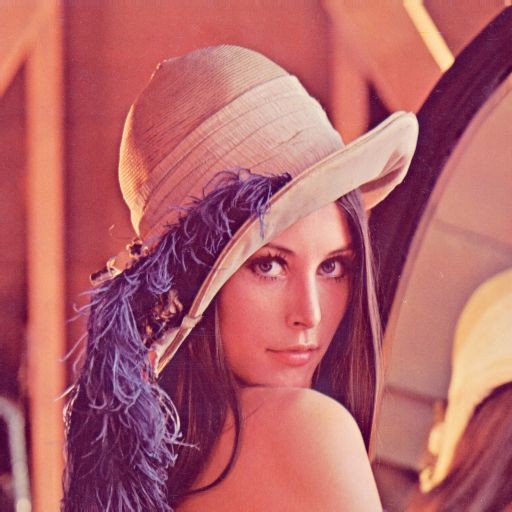
img = read_image("./TestData/lena_color.jpg")
print(img)
write_image("copy_of_lena_color.jpg", img)
Point cloud
ポイントクラウド(点群)ファイルの読み込み(read_point_cloud)、書き込み(write_point_cloud)の関数の紹介:
print("Testing IO for point cloud ...")
pcd = read_point_cloud("./TestData/fragment.pcd")
print(pcd)
write_point_cloud("copy_of_fragment.pcd", pcd)
print() 関数はpcdの内容要約の表示に使える。上記の結果表示されるメッセージは:
Testing IO for point cloud ...
PointCloud with 113662 points.
Mesh
メッシュの読み込み(read_triangle_mesh)と書き込み(write_triangle_mesh)の関数の紹介:
print("Testing IO for meshes ...")
mesh = read_triangle_mesh("./TestData/knot.ply")
print(mesh)
write_triangle_mesh("copy_of_knot.ply", mesh)
ポイントクラウド(点群)とは異なり、メッシュは表面を定義する三角形の集まり、というデータ構造を持つ。
Image
画像の読み込み(read_image)と書き込み(write_image)の関数の紹介:
print("Testing IO for images ...")
img = read_image("./TestData/lena_color.jpg")
print(img)
write_image("copy_of_lena_color.jpg", img)
print関数により、画像のサイズが表示される:
Testing IO for images ...
Image of size 512x512, with 3 channels.
Use numpy.asarray to access buffer data.Point Cloud
ポイントクラウド(点群)の使い方
参考: ポイントクラウドの可視化プログラムとしてPCL提供のもの以外に、http://www.danielgm.net/cc/ がある。Ubuntuではsnap install cloudcompare によってインストールが可能。`cloudcompare.CloudCompare'で起動 (紹介記事: http://www.pointcloud.jp/blog_n23/)
# src/Python/Tutorial/Basic/pointcloud.py
import numpy as np
from py3d import *
if __name__ == "__main__":
print("Load a ply point cloud, print it, and render it")
pcd = read_point_cloud("./TestData/fragment.ply")
print(pcd)
print(np.asarray(pcd.points))
draw_geometries([pcd])
print("Downsample the point cloud with a voxel of 0.05")
downpcd = voxel_down_sample(pcd, voxel_size = 0.05)
draw_geometries([downpcd])
print("Recompute the normal of the downsampled point cloud")
estimate_normals(downpcd, search_param = KDTreeSearchParamHybrid(
radius = 0.1, max_nn = 30))
draw_geometries([downpcd])
print("")
print("Load a polygon volume and use it to crop the original point cloud")
vol = read_selection_polygon_volume("./TestData/Crop/cropped.json")
chair = vol.crop_point_cloud(pcd)
draw_geometries([chair])
print("")
print("Paint chair")
chair.paint_uniform_color([1, 0.706, 0])
draw_geometries([chair])
print("")
Visualize point cloud
はじめに、ポイントクラウド(点群)ファイルを読み込み、それを可視化する方法を紹介
print("Load a ply point cloud, print it, and render it")
pcd = read_point_cloud("./TestData/fragment.ply")
print(pcd)
print(np.asarray(pcd.points))
draw_geometries([pcd])
read_point_cloud 関数はファイルからポイントクラウドを読み込み、その拡張子に基づいてデコードを試みる。扱える拡張子は: pcd, ply, xyz, xyzrgb, xyzn, pts.
draw_geometries は ポイントクラウドを可視化する。マウスを用いて、いろいろな視点からその幾何形状をみることができる。
みかけは密度のある曲面のようにみえるが、実際にはsurfles(曲面要素)としてレンダリングされたものである。GUIによりいろいろなキーボード関数がサポートされている。そのひとつは、- キーで点群数を小さくする。これを何回か押してみると次のように見えるだろう;

-- Mouse view control --
Left button + drag : Rotate. (回転)
Ctrl + left button + drag : Translate. (平行移動)
Wheel : Zoom in/out. (ズームイン・アウト)
-- Keyboard view control --
[/] : Increase/decrease field of view.
R : Reset view point.
Ctrl/Cmd + C : Copy current view status into the clipboard.
Ctrl/Cmd + V : Paste view status from clipboard.
-- General control --
Q, Esc : Exit window. (終了)
H : Print help message. (ヘルプメッセージの表示)
P, PrtScn : Take a screen capture. (スクリーンキャプチャ)
D : Take a depth capture. (深さキャプチャ)
O : Take a capture of current rendering settings. (現在のレンダリング設定のキャプチャ)
-- Render mode control --
L : Turn on/off lighting.
+/- : Increase/decrease point size.
N : Turn on/off point cloud normal rendering.
S : Toggle between mesh flat shading and smooth shading.
W : Turn on/off mesh wireframe.
B : Turn on/off back face rendering.
I : Turn on/off image zoom in interpolation.
T : Toggle among image render:
no stretch / keep ratio / freely stretch.
-- Color control --
0..4,9 : Set point cloud color option.
0 - Default behavior, render point color.
1 - Render point color.
2 - x coordinate as color.
3 - y coordinate as color.
4 - z coordinate as color.
9 - normal as color.
Ctrl + 0..4,9: Set mesh color option.
0 - Default behavior, render uniform gray color.
1 - Render point color.
2 - x coordinate as color.
3 - y coordinate as color.
4 - z coordinate as color.
9 - normal as color.
Shift + 0..4 : Color map options.
0 - Gray scale color.
1 - JET color map.
2 - SUMMER color map.
3 - WINTER color map.
4 - HOT color map.Voxel downsampling
ボクセル(voxel)の説明: https://ja.wikipedia.org/wiki/%E3%83%9C%E3%82%AF%E3%82%BB%E3%83%AB
ボクセルのダウンサンプリングは、通常のボクセル・グリッドを使用して、入力点群から一様にダウンサンプリングされたポイントクラウド(点群)を作成する。 これは、多くのポイント・クラウド処理タスクの前処理ステップとしてよく使用される。 アルゴリズムは2つのステップで動作する。
- ポイントをボクセルに入れる。
- 占有された各ボクセルは、内部のすべての点を平均化することによって正確な1点を生成する。
print("Downsample the point cloud with a voxel of 0.05")
downpcd = voxel_down_sample(pcd, voxel_size = 0.05)
draw_geometries([downpcd])

Vertex normal estimation
ポイントクラウドに対するもうひとつの基本操作は、点法線推定(point normal estimation)である.
print("Recompute the normal of the downsampled point cloud")
estimate_normals(downpcd, search_param = KDTreeSearchParamHybrid(
radius = 0.1, max_nn = 30))
draw_geometries([downpcd])
print("")
estimate_normalsはすべての点の法線を計算する。 この関数は共分散分析を用いて隣接点を見つけ、隣接点の主軸を計算する。
この関数は、KDTreeSearchParamHybridクラスのインスタンスを引数として取る。 radius = 0.1とmax_nn = 30という2つの重要な引数は、検索半径と最大最近傍を指定するもの。 これにより10cmの探索半径を持ち、計算時間を節約するため最大30個の近傍しか考慮しない。
共分散分析アルゴリズムは、法線の候補として2つの互いに反対方向のベクトルを生成する。 ジオメトリのグローバルな構造を知らなければ、どちらも正しい可能性がある。
これは、法線方向問題として知られている問題である。 Open3Dは、法線が存在する場合、元の法線と揃うように法線の方向付けを試みる。 それ以外の場合、Open3Dはランダムな推測を行う。 方向が重要な場合は、orient_normals_to_align_with_directionやorient_normals_towards_camera_locationなどの方向付け関数を呼び出す必要がある。
draw_geometriesを使用して点群を可視化し、nを押して点の法線を表示する。 -キーと+キーを使用して法線の長さを制御できる。

Crop point cloud
read_selection_polygon_volume はポリゴン選択領域を指定するJSONファイルを読み込む。 vol.crop_point_cloud(pcd)は点群をフィルターする。 以下を実行すると椅子だけが選択されて残る。
print("We load a polygon volume and use it to crop the original point cloud")
vol = read_selection_polygon_volume("./TestData/Crop/cropped.json")
chair = vol.crop_point_cloud(pcd)
draw_geometries([chair])
print("")
./TestData/Crop/cropped.json ファイルの内容:
{
"axis_max" : 4.022921085357666,
"axis_min" : -0.76341366767883301,
"bounding_polygon" :
[
[ 2.6509309513852526, 0.0, 1.6834473132326844 ],
[ 2.5786428246917148, 0.0, 1.6892074266735244 ],
[ 2.4625790337552154, 0.0, 1.6665777078297999 ],
[ 2.2228544982251655, 0.0, 1.6168160446813649 ],
[ 2.166993206001413, 0.0, 1.6115495157201662 ],
[ 2.1167895865303286, 0.0, 1.6257706054969348 ],
[ 2.0634657721747383, 0.0, 1.623021658624539 ],
[ 2.0568612343437236, 0.0, 1.5853892911207643 ],
[ 2.1605399001237027, 0.0, 0.96228993255083017 ],
[ 2.1956669387205228, 0.0, 0.95572746049785073 ],
[ 2.2191318790575583, 0.0, 0.88734449982108754 ],
[ 2.2484881847925919, 0.0, 0.87042807267013633 ],
[ 2.6891234157295827, 0.0, 0.94140677988967603 ],
[ 2.7328692490470647, 0.0, 0.98775740674840251 ],
[ 2.7129337547575547, 0.0, 1.0398850034649203 ],
[ 2.7592174072415405, 0.0, 1.0692940558509485 ],
[ 2.7689216419453428, 0.0, 1.0953914441371593 ],
[ 2.6851455625455669, 0.0, 1.6307334122162018 ],
[ 2.6714776099981239, 0.0, 1.675524657088997 ],
[ 2.6579576128816544, 0.0, 1.6819127849749496 ]
],
"class_name" : "SelectionPolygonVolume",
"orthogonal_axis" : "Y",
"version_major" : 1,
"version_minor" : 0
}実行結果の画像:

Paint point cloud
paint_uniform_color は一様な色で全ての点に色付けする。色はRGB空間 [0, 1] の範囲で指定する。
下記のプログラムの実行結果:

print("Paint chair")
chair.paint_uniform_color([1, 0.706, 0])
draw_geometries([chair])
print("")
Mesh
Open3D には三角メッシュのためのデータ構造がある。
# src/Python/Tutorial/Basic/mesh.py
import numpy as np
import copy
from py3d import *
if __name__ == "__main__":
print("Testing mesh in py3d ...")
mesh = read_triangle_mesh("./TestData/knot.ply")
print(mesh)
print(np.asarray(mesh.vertices))
print(np.asarray(mesh.triangles))
print("")
print("Try to render a mesh with normals (exist: " +
str(mesh.has_vertex_normals()) +
") and colors (exist: " + str(mesh.has_vertex_colors()) + ")")
draw_geometries([mesh])
print("A mesh with no normals and no colors does not seem good.")
print("Computing normal and rendering it.")
mesh.compute_vertex_normals()
print(np.asarray(mesh.triangle_normals))
draw_geometries([mesh])
print("We make a partial mesh of only the first half triangles.")
mesh1 = copy.deepcopy(mesh)
mesh1.triangles = Vector3iVector(
np.asarray(mesh1.triangles)[:len(mesh1.triangles)//2, :])
mesh1.triangle_normals = Vector3dVector(
np.asarray(mesh1.triangle_normals)
[:len(mesh1.triangle_normals)//2, :])
print(mesh1.triangles)
draw_geometries([mesh1])
print("Painting the mesh")
mesh1.paint_uniform_color([1, 0.706, 0])
draw_geometries([mesh1])
Print vertices and triangles
(ノードと三角の表示)
print("Testing mesh in py3d ...")
mesh = read_triangle_mesh("./TestData/knot.ply")
print(mesh)
print(np.asarray(mesh.vertices))
print(np.asarray(mesh.triangles))
print("")
この出力は
TriangleMesh with 1440 points and 2880 triangles.
[[ 4.51268387 28.68865967 -76.55680847]
[ 7.63622284 35.52046967 -69.78063965]
[ 6.21986008 44.22465134 -64.82303619]
...,
[-22.12651634 31.28466606 -87.37570953]
[-13.91188431 25.4865818 -86.25827026]
[ -5.27768707 23.36245346 -81.43279266]]
[[ 0 12 13]
[ 0 13 1]
[ 1 13 14]
...,
[1438 11 1439]
[1439 11 0]
[1439 0 1428]]TriangleMeshクラスには、頂点や三角形などのいくつかのデータフィールドがある。 Open3Dは、numpy配列を介してこれらのフィールドへの直接的なメモリ・アクセスを提供する。
Visualize 3D mesh
3D メッシュの可視化
print("Try to render a mesh with normals (exist: " +
str(mesh.has_vertex_normals()) +
") and colors (exist: " + str(mesh.has_vertex_colors()) + ")")
draw_geometries([mesh])
print("A mesh with no normals and no colors does not seem good.")
Try to render a mesh with normals (exist: False) and colors (exist: False)
A mesh with no normals and no colors does not seem good.これによりメッシュを可視化する。

メッシュを回転したり移動したりすることはできるが、灰色で均一に塗られており、「3d」のように見えない。その理由は、この時点のメッシュに頂点や面の法線がないためである。 したがって、より洗練されたPhongシェーディングの代わりに、均一なカラーシェーディングが使用される。
Surface normal estimation (表面法線推定)
表面法線でメッシュを書くことにしよう。
print("Computing normal, painting the mesh, and rendering it.")
mesh.compute_vertex_normals()
print(np.asarray(mesh.triangle_normals))
draw_geometries([mesh])
Computing normal and rendering it.
[[ 0.79164373 -0.53951444 0.28674793]
[ 0.8319824 -0.53303008 0.15389681]
[ 0.83488162 -0.09250101 0.54260136]
...
[ 0.16269924 -0.76215917 -0.6266118 ]
[ 0.52755226 -0.83707495 -0.14489352]
[ 0.56778973 -0.76467734 -0.30476777]]これはmeshモジュールの関数のcompute_vertex_normalsと paint_uniform_color を用いて次のような表示を行う:

Crop mesh
この三角メッシュとtriangle_normalsデータに直接操作し、半分くらいを削除しよう。それにはnumpy配列を介して行う。
print("We make a partial mesh of only the first half triangles.")
mesh1 = copy.deepcopy(mesh)
mesh1.triangles = Vector3iVector(
np.asarray(mesh1.triangles)[:len(mesh1.triangles)//2, :])
mesh1.triangle_normals = Vector3dVector(
np.asarray(mesh1.triangle_normals)
[:len(mesh1.triangle_normals)//2, :])
print(mesh1.triangles)
draw_geometries([mesh1])
その結果は:
We make a partial mesh of only the first half triangles.
std::vector<Eigen::Vector3i> with 1440 elements.
Use numpy.asarray() to access data.
import numpy as np
np.asarray(mesh)
Paint mesh
メッシュの色付けは、ポイントクラウドと同様に行える。
print("Painting the mesh")
mesh1.paint_uniform_color([1, 0.706, 0])
draw_geometries([mesh1])
その結果:

RGBD Images
Open3Dには画像用のデータ構造がある。 read_image、write_image、filter_image、draw_geometriesなどのさまざまな関数を用意している。 Open3Dイメージは、numpy配列に直接変換することができる。
Open3Dの RGBDImageは、RGBDImage.depthとRGBDImage.colorの2つの画像で構成されている。 ただし2つの画像を同じカメラフレームで位置合わせし、同じ解像度にする必要がある。 以下のチュートリアルでは、よく知られているいくつかのRGBDデータセットからRGBDイメージを読み込んで使用する方法を示す。
Redwood dataset
ここでは Redwoodデータセット Choi et al.(2015)からGBDImageを読み込み、可視化する。
- Choi, S., Zhou, Q.-Y., & V. Koltun. (2015). Robust Reconstruction of Indoor Scenes, CVPR.
# src/Python/Tutorial/Basic/rgbd_redwood.py
%matplotlib inline
#conda install pillow matplotlib
from py3d import *
import matplotlib.pyplot as plt
if __name__ == "__main__":
print("Read Redwood dataset")
color_raw = read_image("./TestData/RGBD/color/00000.jpg")
depth_raw = read_image("./TestData/RGBD/depth/00000.png")
rgbd_image = create_rgbd_image_from_color_and_depth(
color_raw, depth_raw);
print(rgbd_image)
plt.figure(figsize=(12,5))
plt.subplot(1, 3, 1)
plt.title('Redwood original image')
plt.imshow(color_raw)
plt.subplot(1, 3, 2)
plt.title('Redwood grayscale image')
plt.imshow(rgbd_image.color, cmap='gray')
plt.subplot(1, 3, 3)
plt.title('Redwood depth image')
plt.imshow(rgbd_image.depth)
plt.show()
pcd = create_point_cloud_from_rgbd_image(rgbd_image,
PinholeCameraIntrinsic.prime_sense_default)
# Flip it, otherwise the pointcloud will be upside down
pcd.transform([[1, 0, 0, 0], [0, -1, 0, 0], [0, 0, -1, 0], [0, 0, 0, 1]])
draw_geometries([pcd])

(Getting Startedでみたデータと同じ)
Redwoodフォーマットは、16ビットのシングルチャンネル画像に深度を格納している。 整数値はミリメートル単位の深度測定値を表す。 Open3Dが奥行き画像を解析するためのデフォルトのフォーマットである。
print("Read Redwood dataset")
color_raw = read_image("./TestData/RGBD/color/00000.jpg")
depth_raw = read_image("./TestData/RGBD/depth/00000.png")
rgbd_image = create_rgbd_image_from_color_and_depth(
color_raw, depth_raw);
print(rgbd_image)
デフォルトの変換関数create_rgbd_image_from_color_and_depthは、色と奥行き画像のペアからRGBDImageを作成する。 カラー画像はグレースケール画像に変換され、[0、1]の範囲のfloatに格納される。 奥行き画像は、深度値をメートルで表した浮動小数点数で格納さる。 print(rgbd_image)は以下を表示する:
RGBDImage of size
Color image : 640x480, with 1 channels.
Depth image : 640x480, with 1 channels.
Use numpy.asarray to access buffer data.変換された画像は、numpy配列としてレンダリングすることができる。
plt.subplot(1, 2, 1)
plt.title('Redwood grayscale image')
plt.imshow(rgbd_image.color)
plt.subplot(1, 2, 2)
plt.title('Redwood depth image')
plt.imshow(rgbd_image.depth)
plt.show()
RGBD画像は、カメラ・パラメータにより、ポイントクラウド(点群)に変換することができる。
pcd = create_point_cloud_from_rgbd_image(rgbd_image,
                PinholeCameraIntrinsic.prime_sense_default)
# Flip it, otherwise the pointcloud will be upside down
pcd.transform([[1, 0, 0, 0], [0, -1, 0, 0], [0, 0, -1, 0], [0, 0, 0, 1]])
draw_geometries([pcd])
ここでは、デフォルトのカメラ・パラメータとしてPinholeCameraIntrinsic.prime_sense_defaultを使用する。 画像の解像度は640x480、焦点距離(fx、fy)=(525.0,525.0)、光学中心(cx、cy)=(319.5,239.5)である。 恒等行列(単位行列)がデフォルトの外部パラメータとして使用される。 pcd.transformは、わかりやすい視点にするため、ポイントクラウド上で上下反転変換を適用する。 この結果は:

SUN dataset
ここではSUN dataset (Song et al. 2015)を読み、可視化する。
Song,S., Lichtenberg, S. & J. Xiao (2015). SUN RGB-D: A RGB-D Scene Understanding Benchmark Suite, CVPR.
# src/Python/Tutorial/Basic/rgbd_sun.py
%matplotlib inline
#conda install pillow matplotlib
from py3d import *
import matplotlib.pyplot as plt


if __name__ == "__main__":
        print("Read SUN dataset")
        color_raw = read_image("./TestData/RGBD/other_formats/SUN_color.jpg")
        depth_raw = read_image("./TestData/RGBD/other_formats/SUN_depth.png")
        rgbd_image = create_rgbd_image_from_sun_format(color_raw, depth_raw);
        print(rgbd_image)
        plt.figure(figsize=(12,5))
        plt.subplot(1, 3, 1)
        plt.title('SUN original image')
        plt.imshow(color_raw)
        plt.subplot(1, 3,  2)
        plt.title('SUN grayscale image')
        plt.imshow(rgbd_image.color, cmap='gray')
        plt.subplot(1, 3, 3)
        plt.title('SUN depth image')
        plt.imshow(rgbd_image.depth)
        plt.show()
        pcd = create_point_cloud_from_rgbd_image(rgbd_image,
                        PinholeCameraIntrinsic.prime_sense_default)
        # Flip it, otherwise the pointcloud will be upside down
        pcd.transform([[1, 0, 0, 0], [0, -1, 0, 0], [0, 0, -1, 0], [0, 0, 0, 1]])
        draw_geometries([pcd])

このチュートリアルは、Redwoodデータセットを処理するチュートリアルとほぼ同じであるが、唯一の違いは、変換関数create_rgbd_image_from_sun_formatを使用して、SUNデータセットの深度画像を解析することである。
RGBDImageをnumpy配列としてレンダリングすることもできる:

ポイントクラウドとしても出力できる:

NYU dataset
このチュートリアルは、NYU dataset (Silberman et al. 2012)のRGBDImageを読み込み可視化する。
Silberman, N., Hoiem, D., Kohli, P., & R. Fergus (2012) Indoor Segmentation and Support Inference from RGBD Images, ECCV.
Redwoodデータセットを処理するチュートリアルとほぼ同じであるが、2つの違いがある。 まず、NYUの画像は標準のjpg形式でもpng形式でもない。 したがって、mpimg.imreadを使用してカラー画像を数値配列として読み込み、それをOpen3D Imageに変換する。 追加のヘルパー関数read_nyu_pgmを呼び出し、NYUデータセットで使用される特別なビッグエンディアンのpgm形式から深度イメージを読み込む。 次に、変換関数create_rgbd_image_from_nyu_formatを使用して、SUNデータセットの深度イメージを解析する。
同様に、RGBDImageをnumpy配列としてレンダリングすることもできる:
# src/Python/Tutorial/Basic/rgbd_nyu.py
%matplotlib inline
#conda install pillow matplotlib
from py3d import *
import numpy as np
import re
import matplotlib.image as mpimg
import matplotlib.pyplot as plt

# This is special function used for reading NYU pgm format
# as it is written in big endian byte order.
def read_nyu_pgm(filename, byteorder='>'):
        with open(filename, 'rb') as f:
                buffer = f.read()
        try:
                header, width, height, maxval = re.search(
                        b"(^P5\s(?:\s*#.*[\r\n])*"
                        b"(\d+)\s(?:\s*#.*[\r\n])*"
                        b"(\d+)\s(?:\s*#.*[\r\n])*"
                        b"(\d+)\s(?:\s*#.*[\r\n]\s)*)", buffer).groups()
        except AttributeError:
                raise ValueError("Not a raw PGM file: '%s'" % filename)
        img = np.frombuffer(buffer,
                dtype=byteorder+'u2',
                count=int(width)*int(height),
                offset=len(header)).reshape((int(height), int(width)))
        img_out = img.astype('u2')
        return img_out

if __name__ == "__main__":
        print("Read NYU dataset")
        # Open3D does not support ppm/pgm file yet. Not using read_image here.
        # MathplotImage having some ISSUE with NYU pgm file. Not using imread for pgm.
        color_raw = mpimg.imread("./TestData/RGBD/other_formats/NYU_color.ppm")
        depth_raw = read_nyu_pgm("./TestData/RGBD/other_formats/NYU_depth.pgm")
        color = Image(color_raw)
        depth = Image(depth_raw)
        rgbd_image = create_rgbd_image_from_nyu_format(color, depth)
        print(rgbd_image)
        plt.figure(figsize=(12,5))
        plt.subplot(1,3,1)
        plt.title('NYU original image')
        plt.imshow(color_raw)
        plt.subplot(1, 3, 2)
        plt.title('NYU grayscale image')
        plt.imshow(rgbd_image.color,cmap='gray')
        plt.subplot(1, 3, 3)
        plt.title('NYU depth image')
        plt.imshow(rgbd_image.depth)
        plt.show()
        pcd = create_point_cloud_from_rgbd_image(rgbd_image,
                        PinholeCameraIntrinsic.prime_sense_default)
        # Flip it, otherwise the pointcloud will be upside down
        pcd.transform([[1, 0, 0, 0], [0, -1, 0, 0], [0, 0, -1, 0], [0, 0, 0, 1]])
        draw_geometries([pcd])

ポイントクラウドとしての表示:

TUM dataset
TUM dataset (Strum et al. 2012)を用いた紹介。
Sturm, J., Engelhard, N., Endres, F., Burgard W., & D. Cremers (2012) A Benchmark for the Evaluation of RGB-D SLAM Systems, IROS.
これもRedwoodデータセットを処理するチュートリアルとほぼ同じであるが、唯一の違いは、変換関数create_rgbd_image_from_tum_formatを使用して、TUMデータセットの深度画像を解析することである。Redwoodデータセットと同様に、RGBDImageをnumpy配列としてレンダリングすることもできる。
# src/Python/Tutorial/Basic/rgbd_tum.py
#conda install pillow matplotlib
%matplotlib inline
from py3d import *
import matplotlib.pyplot as plt


if __name__ == "__main__":
        print("Read TUM dataset")
        color_raw = read_image("./TestData/RGBD/other_formats/TUM_color.png")
        depth_raw = read_image("./TestData/RGBD/other_formats/TUM_depth.png")
        rgbd_image = create_rgbd_image_from_tum_format(color_raw, depth_raw);
        print(rgbd_image)
        plt.figure(figsize=(12,5))
        plt.subplot(1,3,1)
        plt.title('TUM original image')
        plt.imshow(color_raw)
        plt.subplot(1, 3, 2)
        plt.title('TUM grayscale image')
        plt.imshow(rgbd_image.color, cmap='gray')
        plt.subplot(1, 3, 3)
        plt.title('TUM depth image')
        plt.imshow(rgbd_image.depth)
        plt.show()
        pcd = create_point_cloud_from_rgbd_image(rgbd_image,
                        PinholeCameraIntrinsic.prime_sense_default)
        # Flip it, otherwise the pointcloud will be upside down
        pcd.transform([[1, 0, 0, 0], [0, -1, 0, 0], [0, 0, -1, 0], [0, 0, 0, 1]])
        draw_geometries([pcd])

ポイントクラウドとしての表示:

RGBD odometry
RGBDオドメトリは、2つの連続するRGBD画像対の間でカメラの動きを見つける。 入力はRGBDImageの2つのインスタンスで、 出力は剛体変換の形の動きである。 Open3Dは、Steinbrucker et al.(2011)とPark et al.(2017)という2つのRGBDオドメトリを実装している。
Steinbrucker, F., Sturm, J., & D. Cremers (2011). Real-time visual odometry from dense RGB-D images, In ICCV Workshops.
Park, J., Zhou, Q.-Y., & V. Koltun. (2017) Colored Point Cloud Registration Revisited, ICCV.
from py3d import *
import numpy as np

if __name__ == "__main__":
    pinhole_camera_intrinsic = read_pinhole_camera_intrinsic(
            "./TestData/camera.json")
    print(pinhole_camera_intrinsic.intrinsic_matrix)

    source_color = read_image("./TestData/RGBD/color/00000.jpg")
    source_depth = read_image("./TestData/RGBD/depth/00000.png")
    target_color = read_image("./TestData/RGBD/color/00001.jpg")
    target_depth = read_image("./TestData/RGBD/depth/00001.png")
    source_rgbd_image = create_rgbd_image_from_color_and_depth(
            source_color, source_depth);
    target_rgbd_image = create_rgbd_image_from_color_and_depth(
            target_color, target_depth);
    target_pcd = create_point_cloud_from_rgbd_image(
            target_rgbd_image, pinhole_camera_intrinsic)

    option = OdometryOption()
    odo_init = np.identity(4)
    print(option)

    [success_color_term, trans_color_term, info] = compute_rgbd_odometry(
            source_rgbd_image, target_rgbd_image,
            pinhole_camera_intrinsic, odo_init,
            RGBDOdometryJacobianFromColorTerm(), option)
    [success_hybrid_term, trans_hybrid_term, info] = compute_rgbd_odometry(
            source_rgbd_image, target_rgbd_image,
            pinhole_camera_intrinsic, odo_init,
            RGBDOdometryJacobianFromHybridTerm(), option)

    if success_color_term:
        print("Using RGB-D Odometry")
        print(trans_color_term)
        source_pcd_color_term = create_point_cloud_from_rgbd_image(
                source_rgbd_image, pinhole_camera_intrinsic)
        source_pcd_color_term.transform(trans_color_term)
        draw_geometries([target_pcd, source_pcd_color_term])
    if success_hybrid_term:
        print("Using Hybrid RGB-D Odometry")
        print(trans_hybrid_term)
        source_pcd_hybrid_term = create_point_cloud_from_rgbd_image(
                source_rgbd_image, pinhole_camera_intrinsic)
        source_pcd_hybrid_term.transform(trans_hybrid_term)
        draw_geometries([target_pcd, source_pcd_hybrid_term])
pinhole_camera_intrinsic = read_pinhole_camera_intrinsic(
        "./TestData/camera.json")
print(pinhole_camera_intrinsic.intrinsic_matrix)
これにより次の表示がなされる:
[[ 415.69219382    0.          319.5       ]
 [   0.          415.69219382  239.5       ]
 [   0.            0.            1.        ]]
注:Open3Dの小さなデータ構造の多くは、jsonファイルから読み書きできる。 これには、カメラの組み込み関数、カメラの軌跡、ポーズグラフなどが含まれる。
Read RGBD image
(RGBD画像の読み込み)
source_color = read_image("./TestData/RGBD/color/00000.jpg")
source_depth = read_image("./TestData/RGBD/depth/00000.png")
target_color = read_image("./TestData/RGBD/color/00001.jpg")
target_depth = read_image("./TestData/RGBD/depth/00001.png")
source_rgbd_image = create_rgbd_image_from_color_and_depth(
        source_color, source_depth)
target_rgbd_image = create_rgbd_image_from_color_and_depth(
        target_color, target_depth)
このコードブロックは、Redwood形式の2組のRGBD画像を読み取る。 この説明についてはRedwoodのデータセットを参照せよ。
注意: Open3Dでは、カラー画像と奥行き画像が同期して同じ座標系に位置合わせされているものと仮定している。 これは、通常、RGBDカメラ設定の同期機能と位置合わせ機能の両方をオンにすることで実行できる
Compute odometry from two RGBD image pairs
(RGBD画像ペアからの距離計算)
[success, trans_color_term, info] = compute_rgbd_odometry(
        source_rgbd_image, target_rgbd_image,
        pinhole_camera_intrinsic, odo_init,
        RGBDOdometryJacobianFromColorTerm(), option)
[success, trans_hybrid_term, info] = compute_rgbd_odometry(
        source_rgbd_image, target_rgbd_image,
        pinhole_camera_intrinsic, odo_init,
        RGBDOdometryJacobianFromHybridTerm(), option)
このコードブロックは、2つの異なるRGBDオドメトリメソッドを呼び出す。 最初のものはSteinbrucker et al.(2011)である。 整列した画像の写真の一貫性を最小限に抑える。 もう一つはPark et al.(2017)で、写真の一貫性に加えて、ジオメトリの制約も実装されている。 どちらの機能も同様の速度で動作する。 しかし、Park et al.(2017)のほうがベンチマークデータセットのテストにおいて精度が高いので、それをお勧めする。
Steinbrucker, F., Sturm, J., & D. Cremers (2011). Real-time visual odometry from dense RGB-D images, In ICCV Workshops.
Park, J., Zhou, Q.-Y., & V. Koltun. (2017) Colored Point Cloud Registration Revisited, ICCV.
Visualize RGBD image pairs
(RGBD画像ペアの可視化)
if success_color_term:
    print("Using RGB-D Odometry")
    print(trans_color_term)
    source_pcd_color_term = create_point_cloud_from_rgbd_image(
            source_rgbd_image, pinhole_camera_intrinsic)
    source_pcd_color_term.transform(trans_color_term)
    draw_geometries([target_pcd, source_pcd_color_term])
if success_hybrid_term:
    print("Using Hybrid RGB-D Odometry")
    print(trans_hybrid_term)
    source_pcd_hybrid_term = create_point_cloud_from_rgbd_image(
            source_rgbd_image, pinhole_camera_intrinsic)
    source_pcd_hybrid_term.transform(trans_hybrid_term)
    draw_geometries([target_pcd, source_pcd_hybrid_term])
RGBD画像ペアは点群に変換され、一緒にレンダリングされる。 第1の(ソース)RGBD画像を表す点群は、オドメトリによって推定された変換で変換されることに留意されたい。 この変換の後、両方の点群が整列する。
出力:
Using RGB-D Odometry
[[  9.99985131e-01  -2.26255547e-04  -5.44848980e-03  -4.68289761e-04]
 [  1.48026964e-04   9.99896965e-01  -1.43539723e-02   2.88993731e-02]
 [  5.45117608e-03   1.43529524e-02   9.99882132e-01   7.82593526e-04]
 [  0.00000000e+00   0.00000000e+00   0.00000000e+00   1.00000000e+00]]
出力:
Using Hybrid RGB-D Odometry
[[  9.99994666e-01  -1.00290715e-03  -3.10826763e-03  -3.75410348e-03]
 [  9.64492959e-04   9.99923448e-01  -1.23356675e-02   2.54977516e-02]
 [  3.12040122e-03   1.23326038e-02   9.99919082e-01   1.88139799e-03]
 [  0.00000000e+00   0.00000000e+00   0.00000000e+00   1.00000000e+00]]
Visualization
可視化
# src/Python/Tutorial/Basic/visualization.py

import sys, copy
import numpy as np
from py3d import *

if __name__ == "__main__":

    print("Load a ply point cloud, print it, and render it")
    pcd = read_point_cloud("./TestData/fragment.ply")
    draw_geometries([pcd])

    print('Lets draw some primitives')
    mesh_sphere = create_mesh_sphere(radius = 1.0)
    mesh_sphere.compute_vertex_normals()
    mesh_sphere.paint_uniform_color([0.1, 0.1, 0.7])
    mesh_cylinder = create_mesh_cylinder(radius = 0.3, height = 4.0)
    mesh_cylinder.compute_vertex_normals()
    mesh_cylinder.paint_uniform_color([0.1, 0.9, 0.1])
    mesh_frame = create_mesh_coordinate_frame(size = 0.6, origin = [-2, -2, -2])

    print("We draw a few primitives using collection.")
    draw_geometries([mesh_sphere, mesh_cylinder, mesh_frame])

    print("We draw a few primitives using + operator of mesh.")
    draw_geometries([mesh_sphere + mesh_cylinder + mesh_frame])

    print("")
draw_geometries function
print("Load a ply point cloud, print it, and render it")
pcd = read_point_cloud("./TestData/fragment.ply")
draw_geometries([pcd])
Open3Dには、ジオメトリオブジェクト(PointCloud、TriangleMesh、Image)のリストを取得し、レンダリングする便利な可視化のための関数draw_geometriesが用意されている。 可視化では、マウス操作、回転スタイルの変更、スクリーンキャプチャによる回転、平行移動、スケーリングなどの多くの機能を実装している。 ウィンドウ内のhを押すと、機能の包括的なリストが印刷される。
-- Mouse view control --
  Left button + drag        : Rotate.
  Ctrl + left button + drag : Translate.
  Wheel                     : Zoom in/out.

-- Keyboard view control --
  [/]          : Increase/decrease field of view.
  R            : Reset view point.
  Ctrl/Cmd + C : Copy current view status into the clipboard.
  Ctrl/Cmd + V : Paste view status from clipboard.

-- General control --
  Q, Esc       : Exit window.
  H            : Print help message.
  P, PrtScn    : Take a screen capture.
  D            : Take a depth capture.
  O            : Take a capture of current rendering settings.
注:
draw_geometriesに加えて、Open3Dには高度な機能を持つ類似関数のセットがある。draw_geometries_with_custom_animationを使用すると、プログラマはカスタムビュー軌道を定義し、GUIでアニメーションを再生することができる。 draw_geometries_with_animation_callbackおよびdraw_geometries_with_key_callbackは、Pythonコールバック関数を入力として受け入れる。 コールバック関数は、自動アニメーションループまたはキープレスイベントで呼び出される。 詳細については、カスタマイズされた可視化を参照のこと。
Viewpointの記憶
最初、点群は上下逆さまにレンダリングされる:

マウスの左ボタン+ドラッグで視点を調整した後、より良い視点に達することができる:

この視点を保持するには、ctrl cを押す。 視点はクリップボードに保存されたjson文字列に変換される。 カメラを別のビューに移動すると、次のようになる。

ctrl vを押すと元の表示に戻る。
Rendering styles
Open3D visualizerはいくつかのレンダリングスタイルをサポートしている。 たとえば、l を押すと、Phongの照明と単純なカラーレンダリングが切り替わり、 2を押すと、x座標に基づいて着色された点が表示される。

カラーマップは、shift 4を押すなどして調整することもできる。 これにより、ジェットカラーマップがホットカラーマップに変更される。

Geometry primitives
print('Lets draw some primitives')
mesh_sphere = create_mesh_sphere(radius = 1.0)
mesh_sphere.compute_vertex_normals()
mesh_sphere.paint_uniform_color([0.1, 0.1, 0.7])
mesh_cylinder = create_mesh_cylinder(radius = 0.3, height = 4.0)
mesh_cylinder.compute_vertex_normals()
mesh_cylinder.paint_uniform_color([0.1, 0.9, 0.1])
mesh_frame = create_mesh_coordinate_frame(size = 0.6, origin = [-2, -2, -2])
このコードは、create_mesh_sphereおよびcreate_mesh_cylinderを使用して球と円柱を生成する。 球は青で塗られており、シリンダーは緑色で塗装されている。 Phongシェーディングをサポートするために、両方のメッシュに対して法線が計算される(3Dメッシュとサーフェスの法線推定の可視化を参照)。 create_mesh_coordinate_frameを使って原点を(-2、-2、-2)に設定した座標軸を作成することもできる。
Draw multiple geometries
print("We draw a few primitives using collection.")
draw_geometries([mesh_sphere, mesh_cylinder, mesh_frame])

print("We draw a few primitives using + operator of mesh.")
draw_geometries([mesh_sphere + mesh_cylinder + mesh_frame])
draw_geometriesはジオメトリのリストをとり、すべてを一緒にレンダリングする。 別な方法として、TriangleMeshが+演算子をサポートしていることを用いて、複数のメッシュを1つに結合する。一番目のアプローチを推薦する。なぜなら、異なるジオメトリの組み合わせをサポートするからである(例えば、メッシュを点群と並行してレンダリングする)。

KDTree
Open3DはFLANNを使用してKDTreesを構築し、最寄りのものを高速に検索する。
# src/Python/Tutorial/Basic/kdtree.py

import numpy as np
from py3d import *

if __name__ == "__main__":

    print("Testing kdtree in py3d ...")
    print("Load a point cloud and paint it gray.")
    pcd = read_point_cloud("./TestData/Feature/cloud_bin_0.pcd")
    pcd.paint_uniform_color([0.5, 0.5, 0.5])
    pcd_tree = KDTreeFlann(pcd)

    print("Paint the 1500th point red.")
    pcd.colors[1500] = [1, 0, 0]

    print("Find its 200 nearest neighbors, paint blue.")
    [k, idx, _] = pcd_tree.search_knn_vector_3d(pcd.points[1500], 200)
    np.asarray(pcd.colors)[idx[1:], :] = [0, 0, 1]

    print("Find its neighbors with distance less than 0.2, paint green.")
    [k, idx, _] = pcd_tree.search_radius_vector_3d(pcd.points[1500], 0.2)
    np.asarray(pcd.colors)[idx[1:], :] = [0, 1, 0]

    print("Visualize the point cloud.")
    draw_geometries([pcd])
    print("")
ポイントクラウドからKDTreeを構築する
print("Testing kdtree in py3d ...")
print("Load a point cloud and paint it gray.")
pcd = read_point_cloud("./TestData/Feature/cloud_bin_0.pcd")
pcd.paint_uniform_color([0.5, 0.5, 0.5])
pcd_tree = KDTreeFlann(pcd)
このスクリプトは点群を読み取り、KDTreeを構築する。 これは、次の最近傍クエリーの前処理ステップである。
隣接ポイントを見つける
print("Paint the 1500th point red.")
pcd.colors[1500] = [1, 0, 0]
アンカーポイントとして1500番目のポイントを選んで赤く塗りつぶす。
search_knn_vector_3dの使用
print("Find its 200 nearest neighbors, paint blue.")
[k, idx, _] = pcd_tree.search_knn_vector_3d(pcd.points[1500], 200)
np.asarray(pcd.colors)[idx[1:], :] = [0, 0, 1]
関数search_knn_vector_3dは、アンカーポイントのk個の最近傍点のインデックスのリストを返す。 これらの隣接点は青色で塗られている。 pcd.colorsをnumpy配列に変換して、ポイントカラーへの一括アクセスを行い、選択したすべてのポイントに青色[0、0、1]をブロードキャストすることに注意しよう。最初のインデックスはアンカーポイント自体であるため、スキップされている。
search_radius_vector_3dの使用
print("Find its neighbors with distance less than 0.2, paint green.")
[k, idx, _] = pcd_tree.search_radius_vector_3d(pcd.points[1500], 0.2)
np.asarray(pcd.colors)[idx[1:], :] = [0, 1, 0]
同様に、search_radius_vector_3dを使用して、指定された半径よりも小さいアンカーポイントまでの距離を持つすべてのポイントを検索することができる。 これらの点は緑色でぬられている。
print("Visualize the point cloud.")
draw_geometries([pcd])
print("")
その結果は:

注意:
Open3Dは、KNN検索search_knn_vector_3dとRNN検索search_radius_vector_3dの他に、ハイブリッド検索機能search_hybrid_vector_3dを提供している。これは、 与えられた半径よりも小さいアンカーポイントまでの距離を持つk個の最近傍点を返す。 この関数は、KNN検索とRNN検索の基準を結合しており、いくつかの文献でRKNN検索と呼ばれている。 多くの実用的なケースではパフォーマンス上の利点があり、多くのOpen3D関数で頻繁に使用されている。
ICP Registration
このチュートリアルでは、ICP(反復最近接点)位置合わせ(registration)アルゴリズムを示す。 長年にわたり、研究と企業の両方で幾何学的な位置合わせ処理の柱となってきた。 入力は2つのポイントクラウド、つまりソースのポイントクラウドをターゲットのポイントクラウドにおおよそ整列させるための初期変換である。 出力は、入力の2つのポイントクラウドを密接に整列させる洗練された変換である。 ヘルパー関数draw_registration_resultは、位置合わせ処理中のアライメントを可視化する。 このチュートリアルでは、ポイントツーポイントICPとポイントツープレーンICP (Rusinkiewicz & Levoy 2001)という2つのICPバリアントを示す。
Rusinkiewicz, S. & M. Levoy. (2001). Efficient variants of the ICP algorithm. In 3-D Digital Imaging and Modeling.
注: ICPについては https://en.wikipedia.org/wiki/Iterative_closest_point 参照
反復最近接点(ICP)は、2つのポイントクラウドの差を最小限に抑えるために使用されるアルゴリズムである。 ICPは、さまざまなスキャンから2Dまたは3Dサーフェスを再構成したり、ロボットにおいて位置推定したり、最適なパス計画を立てたり(特に滑りやすい地形のためにホイールオドメトリーが信頼性が低い場合)、骨モデルの共同位置合わせなどによく使用される。
# src/Python/Tutorial/Basic/icp_registration.py

def draw_registration_result(source, target, transformation):
    source_temp = copy.deepcopy(source)
    target_temp = copy.deepcopy(target)
    source_temp.paint_uniform_color([1, 0.706, 0])
    target_temp.paint_uniform_color([0, 0.651, 0.929])
    source_temp.transform(transformation)
    draw_geometries([source_temp, target_temp])

if __name__ == "__main__":
    source = read_point_cloud("./TestData/ICP/cloud_bin_0.pcd")
    target = read_point_cloud("./TestData/ICP/cloud_bin_1.pcd")
    threshold = 0.02
    trans_init = np.asarray(
                [[0.862, 0.011, -0.507,  0.5],
                [-0.139, 0.967, -0.215,  0.7],
                [0.487, 0.255,  0.835, -1.4],
                [0.0, 0.0, 0.0, 1.0]])
    draw_registration_result(source, target, trans_init)
    print("Initial alignment")
    evaluation = evaluate_registration(source, target,
            threshold, trans_init)
    print(evaluation)

    print("Apply point-to-point ICP")
    reg_p2p = registration_icp(source, target, threshold, trans_init,
            TransformationEstimationPointToPoint())
    print(reg_p2p)
    print("Transformation is:")
    print(reg_p2p.transformation)
    print("")
    draw_registration_result(source, target, reg_p2p.transformation)

    print("Apply point-to-plane ICP")
    reg_p2l = registration_icp(source, target, threshold, trans_init,
            TransformationEstimationPointToPlane())
    print(reg_p2l)
    print("Transformation is:")
    print(reg_p2l.transformation)
    print("")
    draw_registration_result(source, target, reg_p2l.transformation)
Helper visualization function
def draw_registration_result(source, target, transformation):
    source_temp = copy.deepcopy(source)
    target_temp = copy.deepcopy(target)
    source_temp.paint_uniform_color([1, 0.706, 0])
    target_temp.paint_uniform_color([0, 0.651, 0.929])
    source_temp.transform(transformation)
    draw_geometries([source_temp, target_temp])
この関数は、ターゲットのポイントクラウドを可視化し、ソースのポイントクラウドをアライメント変換で変換する。 ターゲットのポイントクラウドおよびソースのポイントクラウドは、それぞれシアンおよびイエローの色で塗られている。 2つのポイントクラウドが互いに重なり合っているほど、整列結果が良好になる。
注意:
関数transformとpaint_uniform_colorはポイントクラウドを変更するので、copy.deepcopyを呼び出してコピーを作成し、元のポイントクラウドを保護している。
Global registration Input
source = read_point_cloud("./TestData/ICP/cloud_bin_0.pcd")
target = read_point_cloud("./TestData/ICP/cloud_bin_1.pcd")
threshold = 0.02
trans_init = np.asarray(
            [[0.862, 0.011, -0.507,  0.5],
            [-0.139, 0.967, -0.215,  0.7],
            [0.487, 0.255,  0.835, -1.4],
            [0.0, 0.0, 0.0, 1.0]])
draw_registration_result(source, target, trans_init)
このスクリプトは、2つのファイルからソース・ポイントクラウドとターゲット・ポイントクラウドを読み込み、大まかな変換を行う。
注意:初期位置合わせは、通常、グローバル位置合わせアルゴリズムによって得られる。 例については、グローバル位置合わせを参照せよ。

print("Initial alignment")
evaluation = evaluate_registration(source, target,
        threshold, trans_init)
print(evaluation)
関数evaluate_registrationは2つの主要なメトリクスを計算する。 fitnessはオーバーラップエリア(inlier対応数/ターゲット内のポイント数)を測定する。数値が大きいほどほど良い。 inlier_rmseはすべてのinlier対応の(Root Mean Squared Error, 平均二乗誤差平方根)を測定する。 数値が小さいほど良い。
Initial alignment
RegistrationResult with fitness = 0.174723, inlier_rmse = 0.011771,
and correspondence_set size of 34741
Access transformation to get result.
ポイントツーポイントICP
一般に、ICPアルゴリズムは2つのステップを繰り返す:
ターゲット・ポイントクラウド${\bf P}$からの対応集合${\cal K}=\{({\bf p}、{\bf q})\}$と、現在の変換行列${\bf T}$で変換されたソース・ポイントクラウド${\bf Q}$を見つける。
対応集合${\cal K}$に対して定義された目的関数$E({\bf T})$を最小化することによって変換${\bf T}$を更新する。 異なるICPの変形は、異なる目的関数$E({\bf T})$)(Besl & McKay (1992), Chen & Medioni(1992), Park et al. (2017) を使用する。
最初に、次の目的関数を用いたポイントツーポイントICP(点対点ICP)アルゴリズム(Besl & McKay 1992)を示す: $\displaystyle E({\bf T}) = \sum_{({\bf p},{\bf q}) \in {\cal K}} \|{\bf p} - {\bf Tq}\|^2$
Besl P. J. & N. D. McKay. (1992) A Method for Registration of 3D Shapes, PAMI.
Chen, Y. & G. G. Medioni (1992) Object modelling by registration of multiple range images, Image and Vision Computing, 10(3).
Park, J., Zhou, Q.-Y., & V. Koltun. (2017) Colored Point Cloud Registration Revisited, ICCV.
print("Apply point-to-point ICP")
reg_p2p = registration_icp(source, target, threshold, trans_init,
        TransformationEstimationPointToPoint())
print(reg_p2p)
print("Transformation is:")
print(reg_p2p.transformation)
print("")
draw_registration_result(source, target, reg_p2p.transformation)
クラスTransformationEstimationPointToPointは、ポイントツーポイントICP対象の残差行列とヤコビ行列を計算する関数を提供する。 関数registration_icpはそれをパラメータとして取り、ポイントツーポイントICPを実行して結果を返す。

Apply point-to-point ICP
RegistrationResult with fitness = 0.372450, inlier_rmse = 0.007760,
and correspondence_set size of 74056
Access transformation to get result.
Transformation is:
[[ 0.83924644  0.01006041 -0.54390867  0.64639961]
 [-0.15102344  0.96521988 -0.21491604  0.75166079]
 [ 0.52191123  0.2616952   0.81146378 -1.50303533]
 [ 0.          0.          0.          1.        ]]
fitnessスコアは0.174723から0.372450に増加し、inlier_rmseは0.011771から0.007760に減少する。 デフォルトでは、registration_icpは収束するまで、または最大反復回数(デフォルトでは30)に達するまで実行される。 より多く計算時間をかけることによって、結果を改善するように変更することができる。
reg_p2p = registration_icp(source, target, threshold, trans_init,
        TransformationEstimationPointToPoint(),
        ICPConvergenceCriteria(max_iteration = 2000))
出力:

Apply point-to-point ICP
RegistrationResult with fitness = 0.621123, inlier_rmse = 0.006583,
and correspondence_set size of 123501
Access transformation to get result.
Transformation is:
[[ 0.84024592  0.00687676 -0.54241281  0.6463702 ]
 [-0.14819104  0.96517833 -0.21706206  0.81180074]
 [ 0.52111439  0.26195134  0.81189372 -1.48346821]
 [ 0.          0.          0.          1.        ]]
ICPアルゴリズムは収束するまで144反復を要した。 最終的なアライメントはタイトで、fitnessスコアは0.621123に向上し、inlier_rmseは0.006583に減少した。
ポイントツープレーンICP
ポイントツープレーンICP(点対平面ICP)アルゴリズム(Chen & Medioni 1992)は、ポイントツーポイントICPとは異なる目的関数を用いている: $\displaystyle E({\bf T})=\sum_{(p,q) \in {\cal K}} (({\bf p}−{\bf Tq})\cdot {\bf n}_p)^2$
ここで、${\bf n}_p$は点${\bf p}$の法線である。 Rusinkiewicz & Levoy(2001)は、ポイントツープレーンICPアルゴリズムの方がポイントツーポイントICPアルゴリズムよりも収束速度が速いことを示している。
Chen Y. & G. G. Medioni. (1992). Object modelling by registration of multiple range images, Image and Vision Computing, 10(3).
Rusinkiewicz, S. & M. Levoy. (2001) Efficient variants of the ICP algorithm. In 3-D Digital Imaging and Modeling.
print("Apply point-to-plane ICP")
reg_p2l = registration_icp(source, target, threshold, trans_init,
        TransformationEstimationPointToPlane())
print(reg_p2l)
print("Transformation is:")
print(reg_p2l.transformation)
print("")
draw_registration_result(source, target, reg_p2l.transformation)
ここではregistration_icpには、別のパラメータTransformationEstimationPointToPlaneが与えられている。 内部的には、このクラスは、ポイントツープレーン(点対平面)ICP対象の残差およびヤコビ行列を計算する関数を実装している。
注意: ポイントツープレーンICPアルゴリズムは点法線を使用する。 このチュートリアルでは、ファイルから法線を読み込んでいる。 法線が与えられていない場合は、頂点の法線推定で計算できる。

Apply point-to-plane ICP
RegistrationResult with fitness = 0.620972, inlier_rmse = 0.006581,
and correspondence_set size of 123471
Access transformation to get result.
Transformation is:
[[ 0.84023324  0.00618369 -0.54244126  0.64720943]
 [-0.14752342  0.96523919 -0.21724508  0.81018928]
 [ 0.52132423  0.26174429  0.81182576 -1.48366001]
 [ 0.          0.          0.          1.        ]]
ポイントツープレーンICPは、30回の反復で緊密なアライメントに達する(適合度0.620972およびinlier_rmse 0.006581)。
NumPyを用いた処理
Open3Dのデータ構造は、NumPyと互換性がある。 このチュートリアルでは、NumPyを使用してsinc関数を作り、Open3Dを使用してその関数を可視化する。
# src/Python/Tutorial/Basic/working_with_numpy.py

import sys, copy
import numpy as np
from py3d import *

if __name__ == "__main__":

    # generate some neat n times 3 matrix using a variant of sync function
    x = np.linspace(-3, 3, 401)
    mesh_x, mesh_y = np.meshgrid(x,x)
    z = np.sinc((np.power(mesh_x,2)+np.power(mesh_y,2)))
    xyz = np.zeros((np.size(mesh_x),3))
    xyz[:,0] = np.reshape(mesh_x,-1)
    xyz[:,1] = np.reshape(mesh_y,-1)
    xyz[:,2] = np.reshape(z,-1)
    print('xyz')
    print(xyz)

    # Pass xyz to Open3D.PointCloud and visualize
    pcd = PointCloud()
    pcd.points = Vector3dVector(xyz)
    write_point_cloud("./TestData/sync.ply", pcd)

    # Load saved point cloud and transform it into NumPy array
    pcd_load = read_point_cloud("./TestData/sync.ply")
    xyz_load = np.asarray(pcd_load.points)
    print('xyz_load')
    print(xyz_load)

    # visualization
    draw_geometries([pcd_load])
上記のコードの最初の部分では $n \times 3$の行列xyzを生成している。その各列は$\displaystyle z = \frac{\sin(x^2+y^2)}{x^2+y^2}$という関係のx,y,zの値をもつ。
NumPyからOpen3Dへ
# Pass xyz to Open3D.PointCloud.points and visualize
pcd = PointCloud()
pcd.points = Vector3dVector(xyz)
write_point_cloud("./TestData/sync.ply", pcd)
Open3Dは、NumPy行列から3Dベクトルへの変換を提供している。 Vector3dVectorを使用すると、NumPy行列をpy3d.PointCloud.pointsに直接割り当てることができる。
このようにして、py3d.PointCloud.colorsやpy3d.PointCloud.normalsなど、類似したデータ構造は、NumPyを使用して割り当てたり変更したりできる。 上記のスクリプトは、ポイントクラウドpcdを次のステップのためのPLYファイルとして保存している(拡張子が ply になっていることに注意)。
注: PLYについてはhttps://ja.wikipedia.org/wiki/PLY_(%E3%83%95%E3%82%A1%E3%82%A4%E3%83%AB%E5%BD%A2%E5%BC%8F)
Open3DからNumPyへ
# Load saved point cloud and transform it into NumPy array
pcd_load = read_point_cloud("./TestData/sync.ply")
xyz_load = np.asarray(pcd_load.points)
print('xyz_load')
print(xyz_load)

# visualization
draw_geometries([pcd_load])
この例が示すように、Vector3dVectorはnp.asarrayを使用してNumPy配列に変換される。
上記のスクリプトは2つの同一の行列を出力する(比較せよ)。
xyz
[[-3.00000000e+00 -3.00000000e+00 -3.89817183e-17]
 [-2.98500000e+00 -3.00000000e+00 -4.94631078e-03]
 [-2.97000000e+00 -3.00000000e+00 -9.52804798e-03]
 ...
 [ 2.97000000e+00  3.00000000e+00 -9.52804798e-03]
 [ 2.98500000e+00  3.00000000e+00 -4.94631078e-03]
 [ 3.00000000e+00  3.00000000e+00 -3.89817183e-17]]
Writing PLY: [========================================] 100%
Reading PLY: [========================================] 100%
xyz_load
[[-3.00000000e+00 -3.00000000e+00 -3.89817183e-17]
 [-2.98500000e+00 -3.00000000e+00 -4.94631078e-03]
 [-2.97000000e+00 -3.00000000e+00 -9.52804798e-03]
 ...
 [ 2.97000000e+00  3.00000000e+00 -9.52804798e-03]
 [ 2.98500000e+00  3.00000000e+00 -4.94631078e-03]
 [ 3.00000000e+00  3.00000000e+00 -3.89817183e-17]]
そして、関数の可視化を行う:

色付きポイントクラウド位置合わせ
このチュートリアルでは、位置合わせにジオメトリとカラーの両方を使用するICPを示す。 Park et al.(2017)のアルゴリズムを実装している。 色情報は、接平面上の位置合わせを固定する。 したがって、このアルゴリズムは、従来のポイントクラウド位置合わせアルゴリズムよりも正確で頑健であり、実行速度はICP位置合わせアルゴリズムに匹敵する。 このチュートリアルでは、ICP位置合わせの表記法を使用する。
Park, J., Zhou, Q.-Y., & V. Koltun (2017) Colored Point Cloud Registration Revisited, ICCV,
# src/Python/Tutorial/Advanced/colored_pointcloud_registration.py

import numpy as np
import copy
from py3d import *


def draw_registration_result_original_color(source, target, transformation):
    source_temp = copy.deepcopy(source)
    source_temp.transform(transformation)
    draw_geometries([source_temp, target])


if __name__ == "__main__":

    print("1. Load two point clouds and show initial pose")
    source = read_point_cloud("./TestData/ColoredICP/frag_115.ply")
    target = read_point_cloud("./TestData/ColoredICP/frag_116.ply")

    # draw initial alignment
    current_transformation = np.identity(4)
    draw_registration_result_original_color(
            source, target, current_transformation)

    # point to plane ICP
    current_transformation = np.identity(4);
    print("2. Point-to-plane ICP registration is applied on original point")
    print("   clouds to refine the alignment. Distance threshold 0.02.")
    result_icp = registration_icp(source, target, 0.02,
            current_transformation, TransformationEstimationPointToPlane())
    print(result_icp)
    draw_registration_result_original_color(
            source, target, result_icp.transformation)

    # colored pointcloud registration
     # This is implementation of following paper
     # J. Park, Q.-Y. Zhou, V. Koltun,
     # Colored Point Cloud Registration Revisited, ICCV 2017
    voxel_radius = [ 0.04, 0.02, 0.01 ];
    max_iter = [ 50, 30, 14 ];
    current_transformation = np.identity(4)
    print("3. Colored point cloud registration")
    for scale in range(3):
        iter = max_iter[scale]
        radius = voxel_radius[scale]
        print([iter,radius,scale])

        print("3-1. Downsample with a voxel size %.2f" % radius)
        source_down = voxel_down_sample(source, radius)
        target_down = voxel_down_sample(target, radius)

        print("3-2. Estimate normal.")
        estimate_normals(source_down, KDTreeSearchParamHybrid(
                radius = radius * 2, max_nn = 30))
        estimate_normals(target_down, KDTreeSearchParamHybrid(
                radius = radius * 2, max_nn = 30))

        print("3-3. Applying colored point cloud registration")
        result_icp = registration_colored_icp(source_down, target_down,
                radius, current_transformation,
                ICPConvergenceCriteria(relative_fitness = 1e-6,
                relative_rmse = 1e-6, max_iteration = iter))
        current_transformation = result_icp.transformation
        print(result_icp)
    draw_registration_result_original_color(
            source, target, result_icp.transformation)
Helper visualization function
def draw_registration_result_original_color(source, target, transformation):
    source_temp = copy.deepcopy(source)
    source_temp.transform(transformation)
    draw_geometries([source_temp, target])
色付きポイントクラウド間のアラインメントを示すため、draw_registration_result_original_colorによりポイントクラウドを元の色でレンダリングしている。
Input of Colored Point Cloud Registration
print("1. Load two point clouds and show initial pose")
source = read_point_cloud("./TestData/ColoredICP/frag_115.ply")
target = read_point_cloud("./TestData/ColoredICP/frag_116.ply")

# draw initial alignment
current_transformation = np.identity(4)
draw_registration_result_original_color(
        source, target, current_transformation)
このスクリプトは、2つのファイルからソースポイントクラウドとターゲットポイントクラウドを読み込む。 初期値として単位行列を使用している。


Point-to-plane ICP in Colored Point Cloud Registration
# point to plane ICP
current_transformation = np.identity(4);
print("2. Point-to-plane ICP registration is applied on original point")
print("   clouds to refine the alignment. Distance threshold 0.02.")
result_icp = registration_icp(source, target, 0.02,
        current_transformation, TransformationEstimationPointToPlane())
print(result_icp)
draw_registration_result_original_color(
        source, target, result_icp.transformation)
まずベースラインの手法としてPoint-to-Plane ICP (点対平面ICP)を実行する。 以下の可視化では、緑色の三角テクスチャの位置がずれている。 これは、幾何学的制約が2つの平面の滑りを妨げないためである。


Colored point cloud registration
色付きポイントクラウド位置合わせの中核はregistration_colored_icpである。 Park et al.(2017)の後、共同最適化の目的でICP反復を実行する(ポイントツーポイントICPを参照)
$ E({\bf T})=(1-\delta)E_C({\bf T})+\delta E_G({|bf T})$
ここで${\bf T}$は推定される変換行列である。$E_C$と$E_G$ は、それぞれ測光および幾何学項である。$\delta \in [0,1]$は経験的に決定された重みパラメータである。
幾何学項$E_G$は、Point-to-Plane ICP(点対平面ICP)の目的関数と同じである:
$ E_G({\bf T}) = \sum_{({\bf p},{\bf q}) \in {\cal K}} (({\bf p} - {\bf Tq})\cdot {\bf n_p})^2$
ここで${\cal K}$は現在の反復における対応集合で、${\bf n_p}$は${\bf p}$点の法線である。
色の項$E_C$は、点${\bf q}$の色($C({\bf q})$で表す)と${\bf p}$の接平面上の投影点の色との間の差を測定値を返す。
$\displaystyle E_C({\bf T})=\sum_{({\bf p},{\bf q}) \in {\cal K}}(C_{\bf p}({\bf f(Tq)})-C({\bf q}))^2$
ここで、$C_{\bf p}(\cdot)$は${\bf p}$の接平面上で連続的に定義された関数で、事前に計算されたものである。 関数${\bf f}(\cdot)$は、3D点を接平面に投影する。 詳細はPark et al.(2017)を参照のこと。
効率性をさらに向上させるために、Park et al.(2017)は、マルチスケールの位置合わせスキームを提案している。 これは、次のスクリプトで実装されている。
Park, J., Zhou, Q.-Y., & V. Koltun (2017) Colored Point Cloud Registration Revisited, ICCV,
# colored pointcloud registration
# This is implementation of following paper
# J. Park, Q.-Y. Zhou, V. Koltun,
# Colored Point Cloud Registration Revisited, ICCV 2017
voxel_radius = [ 0.04, 0.02, 0.01 ];
max_iter = [ 50, 30, 14 ];
current_transformation = np.identity(4)
print("3. Colored point cloud registration")
for scale in range(3):
    iter = max_iter[scale]
    radius = voxel_radius[scale]
    print([iter,radius,scale])

    print("3-1. Downsample with a voxel size %.2f" % radius)
    source_down = voxel_down_sample(source, radius)
    target_down = voxel_down_sample(target, radius)

    print("3-2. Estimate normal.")
    estimate_normals(source_down, KDTreeSearchParamHybrid(
            radius = radius * 2, max_nn = 30))
    estimate_normals(target_down, KDTreeSearchParamHybrid(
            radius = radius * 2, max_nn = 30))

    print("3-3. Applying colored point cloud registration")
    result_icp = registration_colored_icp(source_down, target_down,
            radius, current_transformation,
            ICPConvergenceCriteria(relative_fitness = 1e-6,
            relative_rmse = 1e-6, max_iteration = iter))
    current_transformation = result_icp.transformation
    print(result_icp)
    draw_registration_result_original_color(
            source, target, result_icp.transformation)
Voxelダウンサンプリングを使用して合計3層のマルチ解像度ポイントクラウドが作成される。 法線は、頂点法線推定で計算される。 位置合わせ関数registration_colored_icpは、粗いものから細かいものまで各レイヤーに対して呼び出される。 lambda_geometricは、全体のエネルギー$\lambda E_G+(1-\lambda)E_C$における$\lambda \in [0,1]$の値を決定するregistration_colored_icpのオプション引数である。
出力は、2つの点群の緊密なアライメントである。 壁の緑色の三角形に注目しよう。


Global registration
ICP位置合わせと色付きポイントクラウド位置合わせの両方は、初期設定として大まかなアラインメントに依存しているため、ローカル位置合わせメソッドとして知られていまる。 このチュートリアルでは、グローバル位置合わせと呼ばれる別のクラスの位置合わせメソッドを示す。 これらのアルゴリズムは、初期化のためのアライメントを必要としない。 通常は、タイトな位置合わせ結果が生成されず、局所メソッドの初期化として使用される。
# src/Python/Tutorial/Advanced/global_registration.py

from py3d import *
import numpy as np
import copy

def draw_registration_result(source, target, transformation):
    source_temp = copy.deepcopy(source)
    target_temp = copy.deepcopy(target)
    source_temp.paint_uniform_color([1, 0.706, 0])
    target_temp.paint_uniform_color([0, 0.651, 0.929])
    source_temp.transform(transformation)
    draw_geometries([source_temp, target_temp])

if __name__ == "__main__":

    print("1. Load two point clouds and disturb initial pose.")
    source = read_point_cloud("./TestData/ICP/cloud_bin_0.pcd")
    target = read_point_cloud("./TestData/ICP/cloud_bin_1.pcd")
    trans_init = np.asarray([[0.0, 1.0, 0.0, 0.0],
                            [1.0, 0.0, 0.0, 0.0],
                            [0.0, 0.0, 1.0, 0.0],
                            [0.0, 0.0, 0.0, 1.0]])
    source.transform(trans_init)
    draw_registration_result(source, target, np.identity(4))

    print("2. Downsample with a voxel size 0.05.")
    source_down = voxel_down_sample(source, 0.05)
    target_down = voxel_down_sample(target, 0.05)

    print("3. Estimate normal with search radius 0.1.")
    estimate_normals(source_down, KDTreeSearchParamHybrid(
            radius = 0.1, max_nn = 30))
    estimate_normals(target_down, KDTreeSearchParamHybrid(
            radius = 0.1, max_nn = 30))

    print("4. Compute FPFH feature with search radius 0.25")
    source_fpfh = compute_fpfh_feature(source_down,
            KDTreeSearchParamHybrid(radius = 0.25, max_nn = 100))
    target_fpfh = compute_fpfh_feature(target_down,
            KDTreeSearchParamHybrid(radius = 0.25, max_nn = 100))

    print("5. RANSAC registration on downsampled point clouds.")
    print("   Since the downsampling voxel size is 0.05, we use a liberal")
    print("   distance threshold 0.075.")
    result_ransac = registration_ransac_based_on_feature_matching(
            source_down, target_down, source_fpfh, target_fpfh, 0.075,
            TransformationEstimationPointToPoint(False), 4,
            [CorrespondenceCheckerBasedOnEdgeLength(0.9),
            CorrespondenceCheckerBasedOnDistance(0.075)],
            RANSACConvergenceCriteria(4000000, 500))
    print(result_ransac)
    draw_registration_result(source_down, target_down,
            result_ransac.transformation)

    print("6. Point-to-plane ICP registration is applied on original point")
    print("   clouds to refine the alignment. This time we use a strict")
    print("   distance threshold 0.02.")
    result_icp = registration_icp(source, target, 0.02,
            result_ransac.transformation,
            TransformationEstimationPointToPlane())
    print(result_icp)
    draw_registration_result(source, target, result_icp.transformation)
Input of Global Registration
print("1. Load two point clouds and disturb initial pose.")
source = read_point_cloud("./TestData/ICP/cloud_bin_0.pcd")
target = read_point_cloud("./TestData/ICP/cloud_bin_1.pcd")
trans_init = np.asarray([[0.0, 1.0, 0.0, 0.0],
                        [1.0, 0.0, 0.0, 0.0],
                        [0.0, 0.0, 1.0, 0.0],
                        [0.0, 0.0, 0.0, 1.0]])
source.transform(trans_init)
draw_registration_result(source, target, np.identity(4))
このスクリプトは、2つのファイルからソースポイントクラウドとターゲットポイントクラウドを読み込む。 それらは変換として単位行列を用い、整列してはいない。

Extract geometric feature
print("2. Downsample with a voxel size 0.05.")
source_down = voxel_down_sample(source, 0.05)
target_down = voxel_down_sample(target, 0.05)

print("3. Estimate normal with search radius 0.1.")
estimate_normals(source_down, KDTreeSearchParamHybrid(
        radius = 0.1, max_nn = 30))
estimate_normals(target_down, KDTreeSearchParamHybrid(
        radius = 0.1, max_nn = 30))

print("4. Compute FPFH feature with search radius 0.25")
source_fpfh = compute_fpfh_feature(source_down,
        KDTreeSearchParamHybrid(radius = 0.25, max_nn = 100))
target_fpfh = compute_fpfh_feature(target_down,
        KDTreeSearchParamHybrid(radius = 0.25, max_nn = 100))
ポイントクラウドをサンプリングして法線を推定し、各ポイントのFPFH特徴量を計算する。 FPFH特徴量は、点の局所的幾何学特性を記述する33次元ベクトルである。 33次元空間における最近傍検索により、似たような局所的幾何学構造を有する点を返すことができる。 詳細はRasu et al.(2009)を参照のこと。
Rusu, R., Blodow, N. & M. Beetz. (2009). Fast Point Feature Histograms (FPFH) for 3D registration, ICRA.
注: FPFH特徴量については http://pointclouds.org/documentation/tutorials/fpfh_estimation.php
RANSAC
print("5. RANSAC registration on down-sampled point clouds.")
print("   Since the downsampling voxel size is 0.05, we use a liberal")
print("   distance threshold 0.075.")
result_ransac = registration_ransac_based_on_feature_matching(
        source_down, target_down, source_fpfh, target_fpfh,
        fpfh, max_correspondence_distance = 0.075,
        TransformationEstimationPointToPoint(False),
        ransac_n = 4,
        [CorrespondenceCheckerBasedOnEdgeLength(0.9),
        CorrespondenceCheckerBasedOnDistance(0.075)],
        RANSACConvergenceCriteria(max_iteration = 4000000, max_validation = 500))
print(result_ransac)
draw_registration_result(source_down, target_down,
        result_ransac.transformation)
グローバル位置合わせにはRANSACを使用します。 各RANSAC反復では、ソースのポイントクラウドからランダムな点が選択される。 ターゲットのポイントクラウド内における対応点は、33次元FPFH特徴量空間内の最も近い近傍を検索することによって検出される。 プルーニング(枝きり)のステップでは、初期段階での誤った一致点を削除するための高速プルーニングアルゴリズムが必要である。
注: RANSACについては https://qiita.com/smurakami/items/14202a83bd13e55d4c09 (OpenCVでも使用されている)
Open3Dは以下のプルーニングアルゴリズムを提供している:
CorrespondenceCheckerBasedOnDistanceは、整列したポイントクラウドがクローズしている(指定された閾値未満)かどうかをチェックする。CorrespondenceCheckerBasedOnEdgeLengthは、ソースとターゲットの対応関係から個別に描画された任意の2つのエッジ(2つの頂点で形成された線)の長さが似ているかどうかをチェックする。このチュートリアルでは、 $\| edge_{source} \| > 0.9 \times \| edge_{target} \|$かつ$| edge{target} | > 0.9 \times | edge{source} | が成り立っているかをチェックCorrespondenceCheckerBasedOnNormalは、対応する頂点の法線同士が整合しているかを調べる。つまり、2つの法線ベクトルの内積を計算し、ラディアン値で指定された閾値と比較する。
プルーニング・ステップを通過したマッチのみが変換を計算するために使用され、変換はポイントクラウド全体で検証される。中核となる機能は、registration_ransac_based_on_feature_matchingである。この関数の最も重要なハイパーパラメータはRANSACConvergenceCriteriaである。これは、RANSAC反復の最大数と検証ステップの最大数を定義する。これらの2つの数値が大きいほど結果はより正確になるが、アルゴリズムに要する時間も長くなる。
我々は Choi(2015) で与えられた経験値に基づいてRANSACパラメータを設定しえいる。結果は次のとおり:

Local refinement
パフォーマンス上の理由から、グローバル位置合わせは、大幅にダウンサンプリングされたポイントクラウドに対してのみ実行される。 結果もタイトなものではない。そこで、アライメントをさらに洗練するために、ポイントツープレーンICPを使用する。
print("6. Point-to-plane ICP registration is applied on original point")
print("   clouds to refine the alignment. This time we use a strict")
print("   distance threshold 0.02.")
result_icp = registration_icp(source, target, 0.02,
        result_ransac.transformation,
        TransformationEstimationPointToPlane())
print(result_icp)
draw_registration_result(source, target, result_icp.transformation)
タイトなアライメントを出力する。 これは完全なペアごとの位置合わせワークフローをまとめたものである。

Multiway Registration
多方向位置合わせとは、グローバル空間内の複数のジオメトリを整列させる処理である。 典型的には、入力は幾何学集合(例えば点群やRGBD画像)$\{ {\bf P}_i \}$である。 出力は、剛体変換$\{ {\bf T}_i\}$のセットであり、変換された点群$\{ {\bf T}_i{\bf P}_i\}$はグローバル空間内で整列される。
Open3Dは、ポーズグラフの最適化による多方向位置合わせを実装し、バックエンドとしてChoi(2015)で提示された技術を実装している。
# src/Python/Tutorial/Advanced/multiway_registration.py

from py3d import *

if __name__ == "__main__":

    set_verbosity_level(VerbosityLevel.Debug)
    pcds = []
    for i in range(3):
        pcd = read_point_cloud(
                "./TestData/ICP/cloud_bin_%d.pcd" % i)
        downpcd = voxel_down_sample(pcd, voxel_size = 0.02)
        pcds.append(downpcd)
    draw_geometries(pcds)

    pose_graph = PoseGraph()
    odometry = np.identity(4)
    pose_graph.nodes.append(PoseGraphNode(odometry))

    n_pcds = len(pcds)
    for source_id in range(n_pcds):
        for target_id in range(source_id + 1, n_pcds):
            source = pcds[source_id]
            target = pcds[target_id]

            print("Apply point-to-plane ICP")
            icp_coarse = registration_icp(source, target, 0.3,
                    np.identity(4),
                    TransformationEstimationPointToPlane())
            icp_fine = registration_icp(source, target, 0.03,
                    icp_coarse.transformation,
                    TransformationEstimationPointToPlane())
            transformation_icp = icp_fine.transformation
            information_icp = get_information_matrix_from_point_clouds(
                    source, target, 0.03, icp_fine.transformation)
            print(transformation_icp)

            # draw_registration_result(source, target, np.identity(4))
            print("Build PoseGraph")
            if target_id == source_id + 1: # odometry case
                odometry = np.dot(transformation_icp, odometry)
                pose_graph.nodes.append(
                        PoseGraphNode(np.linalg.inv(odometry)))
                pose_graph.edges.append(
                        PoseGraphEdge(source_id, target_id,
                        transformation_icp, information_icp, uncertain = False))
            else: # loop closure case
                pose_graph.edges.append(
                        PoseGraphEdge(source_id, target_id,
                        transformation_icp, information_icp, uncertain = True))

    print("Optimizing PoseGraph ...")
    option = GlobalOptimizationOption(
            max_correspondence_distance = 0.03,
            edge_prune_threshold = 0.25,
            reference_node = 0)
    global_optimization(pose_graph,
            GlobalOptimizationLevenbergMarquardt(),
            GlobalOptimizationConvergenceCriteria(), option)

    print("Transform points and display")
    for point_id in range(n_pcds):
        print(pose_graph.nodes[point_id].pose)
        pcds[point_id].transform(pose_graph.nodes[point_id].pose)
    draw_geometries(pcds)
Input of Multiway Registration
set_verbosity_level(VerbosityLevel.Debug)
pcds = []
for i in range(3):
    pcd = read_point_cloud(
            "./TestData/ICP/cloud_bin_%d.pcd" % i)
    downpcd = voxel_down_sample(pcd, voxel_size = 0.02)
    pcds.append(downpcd)
draw_geometries(pcds)
スクリプトの最初の部分で、3つのファイル(cloud_bin_0.pcd, cloud_bin_1.pcd, cloud_bin_2.pcd)からそれぞれポイントクラウドを読み込み、ダウンサンプリングして、一緒に可視化する。 これらは(まだ)整列してはいない。

Build a pose graph
ポーズグラフの作成
pose_graph = PoseGraph()
odometry = np.identity(4)
pose_graph.nodes.append(PoseGraphNode(odometry))

n_pcds = len(pcds)
for source_id in range(n_pcds):
    for target_id in range(source_id + 1, n_pcds):
        source = pcds[source_id]
        target = pcds[target_id]

        print("Apply point-to-plane ICP")
        icp_coarse = registration_icp(source, target, 0.3,
                np.identity(4),
                TransformationEstimationPointToPlane())
        icp_fine = registration_icp(source, target, 0.03,
                icp_coarse.transformation,
                TransformationEstimationPointToPlane())
        transformation_icp = icp_fine.transformation
        information_icp = get_information_matrix_from_point_clouds(
                source, target, 0.03, icp_fine.transformation)
        print(transformation_icp)

        # draw_registration_result(source, target, np.identity(4))
        print("Build PoseGraph")
        if target_id == source_id + 1: # odometry case
            odometry = np.dot(transformation_icp, odometry)
            pose_graph.nodes.append(
                    PoseGraphNode(np.linalg.inv(odometry)))
            pose_graph.edges.append(
                    PoseGraphEdge(source_id, target_id,
                    transformation_icp, information_icp, uncertain = False))
        else: # loop closure case
            pose_graph.edges.append(
                    PoseGraphEdge(source_id, target_id,
                    transformation_icp, information_icp, uncertain = True))
ポーズグラフには、ノードとエッジという2つの重要な要素がある。ノードは、${\bf P_i}$をグローバル空間に変換するポーズ行列${\bf T_i}$に関連付けられた幾何学形状${\bf P_i}$の一部分である。集合${\bf T_i}$は最適化される未知の変数であり、 PoseGraph.nodesはPoseGraphNodeのリストである。グローバル空間を${\bf P_0}$の空間とする。従って、${\bf T_0}$は恒等行列である。他のポーズ行列は、隣接ノード間で変換を累積することによって初期化される。隣接ノードは、通常、大きなオーバーラップを有し、ポイントツープレーンICPで位置合わせすることができる。
ポーズグラフのエッジは、重なっている2つのノード(ジオメトリの一部)を接続する。各エッジは、ソースジオメトリ${\bf P_i}$をターゲットジオメトリ${\bf P_j}$に整列させる変換行列${\bf T_{i,j}}$を含む。このチュートリアルでは、ポイントツープレーンICPを使用して変換を推定する。より複雑なケースでは、このペアごとの位置合わせの問題は、グローバル位置合わせを介して解決する必要がある。
Choi(2015)は、ペアごとの位置合わせがエラーを起こしやすいことを指摘している。誤ったアラインメントのペアの個数は、正しくアライメントされたペアの数を上回る。したがって、ポーズグラフのエッジを2つのクラスに分割する。オドメトリ・エッジは、時間的に近い、隣接するノードを接続する。 ICPのような局所的位置合わせアルゴリズムは、それらを確実に整列させることができる。ループ閉包エッジは、非隣接ノードを接続する。アライメントはグローバル位置合わせによって検出され、信頼性が低くなる。 Open3Dでは、これら2つのエッジのクラスは、PoseGraphEdgeのインスタンス作成時においてuncertainパラメータによって区別する。
ユーザは、変換行列${\bf T_i}$に加えて、各エッジについて情報行列${\bf \Lambda_i}$を設定することができる。関数get_information_matrix_from_point_cloudsを使用して${\bf \Lambda_i}$が設定された場合、このポーズグラフのエッジ上の損失関数は、2つのノード間の対応するセットのRMSE(Root Mean Squared Errovr, 平均二乗誤差平方根)で近似する。詳細はChoi(2015)の式(3)〜(9)とRedwood位置合わせベンチマークを参照のこと。
ここでのスクリプトは3つのノードと3つのエッジを持つポーズグラフを作成する。エッジのうち、2つはオドメト・エッジ(uncertain = False)であり、1つはループ閉包エッジ(uncertain = True)である。
Optimize a pose graph
ポーズグラフの最適化
print("Optimizing PoseGraph ...")
option = GlobalOptimizationOption(
        max_correspondence_distance = 0.03,
        edge_prune_threshold = 0.25,
        reference_node = 0)
global_optimization(pose_graph,
        GlobalOptimizationLevenbergMarquardt(),
        GlobalOptimizationConvergenceCriteria(), option)
Open3Dは関数global_optimizationを使ってポーズグラフの最適化を行う。 2種類の最適化メソッド、GlobalOptimizationGaussNewton とGlobalOptimizationLevenbergMarquardt を選択できる。 後者は収束性が良いので推奨する。 クラスGlobalOptimizationConvergenceCriteriaを使用すると、反復の最大回数とさまざまな最適化パラメータを設定できる。
クラスGlobalOptimizationOptionはいくつかのオプションをとる。 max_correspondence_distanceは対応閾値を決定に用いられ、 edge_prune_thresholdは、外れ値エッジをプルーニングするためのしきい値であり、reference_nodeは、グローバル・スペースとみなされるノードIDでである。
Optimizing PoseGraph ...
[GlobalOptimizationLM] Optimizing PoseGraph having 3 nodes and 3 edges.
Line process weight : 3.745800
[Initial     ] residual : 6.741225e+00, lambda : 6.042803e-01
[Iteration 00] residual : 1.791471e+00, valid edges : 3, time : 0.000 sec.
[Iteration 01] residual : 5.133682e-01, valid edges : 3, time : 0.000 sec.
[Iteration 02] residual : 4.412544e-01, valid edges : 3, time : 0.000 sec.
[Iteration 03] residual : 4.408356e-01, valid edges : 3, time : 0.000 sec.
[Iteration 04] residual : 4.408342e-01, valid edges : 3, time : 0.000 sec.
Delta.norm() < 1.000000e-06 * (x.norm() + 1.000000e-06)
[GlobalOptimizationLM] total time : 0.000 sec.
[GlobalOptimizationLM] Optimizing PoseGraph having 3 nodes and 3 edges.
Line process weight : 3.745800
[Initial     ] residual : 4.408342e-01, lambda : 6.064910e-01
Delta.norm() < 1.000000e-06 * (x.norm() + 1.000000e-06)
[GlobalOptimizationLM] total time : 0.000 sec.
CompensateReferencePoseGraphNode : reference : 0
グローバル最適化は、ポーズグラフに対して2回実行される。 最初のパスは、すべてのエッジを考慮した元のポーズグラフのポーズを最適化し、不確実なエッジ間の誤ったアライメントを識別しようとする。 誤ったアライメントは、小さなラインプロセスの重みを持ち、最初のパスの後で枝刈りされれる。 2回目のパスではグローバルな整合性が確保される。 この例では、すべてのエッジが真のアライメントと見なされるため、2番目のパスは直ちに終了する。
Visualize optimization
最適化の可視化
print("Transform points and display")
for point_id in range(n_pcds):
    print(pose_graph.nodes[point_id].pose)
    pcds[point_id].transform(pose_graph.nodes[point_id].pose)
draw_geometries(pcds)

RGBD integration
RGBD統合
Open3DはスケーラブルなRGBD画像統合アルゴリズムを実装している。 このアルゴリズムは Curless(1996)と Newcombe(2011)で提示された手法に基づいている。 大きなシーンをサポートするために、ElasticReconstructionのIntegraterで導入された階層的なハッシュ構造を使用する。
注意: 元のソースでは実行できない:(1) trajectory_io が見つからない、(2) camera_poses = read_trajectory("./TestData/RGBD/odometry.log")がないため、camera_posesが未定義というエラーになる。
そこで、(1)に対しては、Robust Reconstruction of Indoor Scenes のTrajectory File (.log) FormatページからPythonコードをとってきて(以下に示す)、trajectory_io.py というファイルを作る、(2)は原文にあったコードを追加することで対処した。
# trajectory_io.py

import numpy as np
import numpy.linalg

class CameraPose:
    def __init__(self, meta, mat):
        self.metadata = meta
        self.pose = mat
    def __str__(self):
        return 'Metadata : ' + ' '.join(map(str, self.metadata)) + '\n' + \
            "Pose : " + "\n" + np.array_str(self.pose)

def read_trajectory(filename):
    traj = []
    with open(filename, 'r') as f:
        metastr = f.readline();
        while metastr:
            metadata = map(int, metastr.split())
            mat = np.zeros(shape = (4, 4))
            for i in range(4):
                matstr = f.readline();
                mat[i, :] = np.fromstring(matstr, dtype = float, sep=' \t')
            traj.append(CameraPose(metadata, mat))
            metastr = f.readline()
    return traj

def write_trajectory(traj, filename):
    with open(filename, 'w') as f:
        for x in traj:
            p = x.pose.tolist()
            f.write(' '.join(map(str, x.metadata)) + '\n')
            f.write('\n'.join(' '.join(map('{0:.12f}'.format, p[i])) for i in range(4)))
            f.write('\n')
# src/Python/Tutorial/Advanced/rgbd_integration.py
%matplotlib inline
from trajectory_io import read_trajectory
from py3d import *
import numpy as np

if __name__ == "__main__":
    camera_poses = read_trajectory("./TestData/RGBD/odometry.log")
    volume = ScalableTSDFVolume(voxel_length = 4.0 / 512.0,
            sdf_trunc = 0.04, with_color = True)

    for i in range(len(camera_poses)):
        print("Integrate {:d}-th image into the volume.".format(i))
        color = read_image("./TestData/RGBD/color/{:05d}.jpg".format(i))
        depth = read_image("./TestData/RGBD/depth/{:05d}.png".format(i))
        rgbd = create_rgbd_image_from_color_and_depth(color, depth,
                depth_trunc = 4.0, convert_rgb_to_intensity = False)
        volume.integrate(rgbd, PinholeCameraIntrinsic.prime_sense_default,
                np.linalg.inv(camera_poses[i].pose))

    print("Extract a triangle mesh from the volume and visualize it.")
    mesh = volume.extract_triangle_mesh()
    mesh.compute_vertex_normals()
    draw_geometries([mesh])
Read trajectory from .log file
.logファイルから軌跡(trajectory)を読み込む
camera_poses = read_trajectory("./TestData/RGBD/odometry.log")
このチュートリアルでは、関数read_trajectoryを使用して.logファイルからカメラの軌跡を読み込む。 サンプルの.logファイルの内容は次のとおり。
# src/test/TestData/RGBD/odometry.log
0   0   1
1   0   0   2
0   1   0   2
0   0   1 -0.3
0   0   0   1
1   1   2
0.999988  3.08668e-005  0.0049181  1.99962
-8.84184e-005  0.999932  0.0117022  1.97704
-0.0049174  -0.0117024  0.999919  -0.300486
0  0  0  1
:
TSDF volume integration
TSDF (volumetric truncated signed distance function): https://www.slideshare.net/hirokiwaterfield/30th-dynamicfusion や https://github.com/andyzeng/tsdf-fusion 参照
volume = ScalableTSDFVolume(voxel_length = 4.0 / 512.0,
        sdf_trunc = 0.04, with_color = True)

for i in range(len(camera_poses)):
    print("Integrate {:d}-th image into the volume.".format(i))
    color = read_image("./TestData/RGBD/color/{:05d}.jpg".format(i))
    depth = read_image("./TestData/RGBD/depth/{:05d}.png".format(i))
    rgbd = create_rgbd_image_from_color_and_depth(color, depth,
            depth_trunc = 4.0, convert_rgb_to_intensity = False)
    volume.integrate(rgbd, PinholeCameraIntrinsic.prime_sense_default,
            np.linalg.inv(camera_poses[i].pose))
Open3Dは、UniformTSDFVolumeとScalableTSDFVolumeという2種類のTSDFボリュームを提供している。 後者は階層構造を使用し、より大きなシーンをサポートするので推奨する。
ScalableTSDFVolumeにはいくつかのパラメータがあります。voxel_length = 4.0 / 512.0は、TSDFボリュームの単一のボクセルサイズが$\frac{4.0m}{512.0} = 7.8125mm$であることを意味する。 この値を小さくすると、高解像度のTSDFボリュームになるが、積分結果が深度ノイズの影響を受けやすくなる。 sdf_trunc = 0.04は、符号付き距離関数(SDF, Signed Distance Function)の切り捨て(trancated)値を指定する。 with_color = Trueの場合、色もTSDFボリュームの一部として統合される。 カラーインテグレーションはPCLに触発されたものである。
Extract a mesh
メッシュの抽出
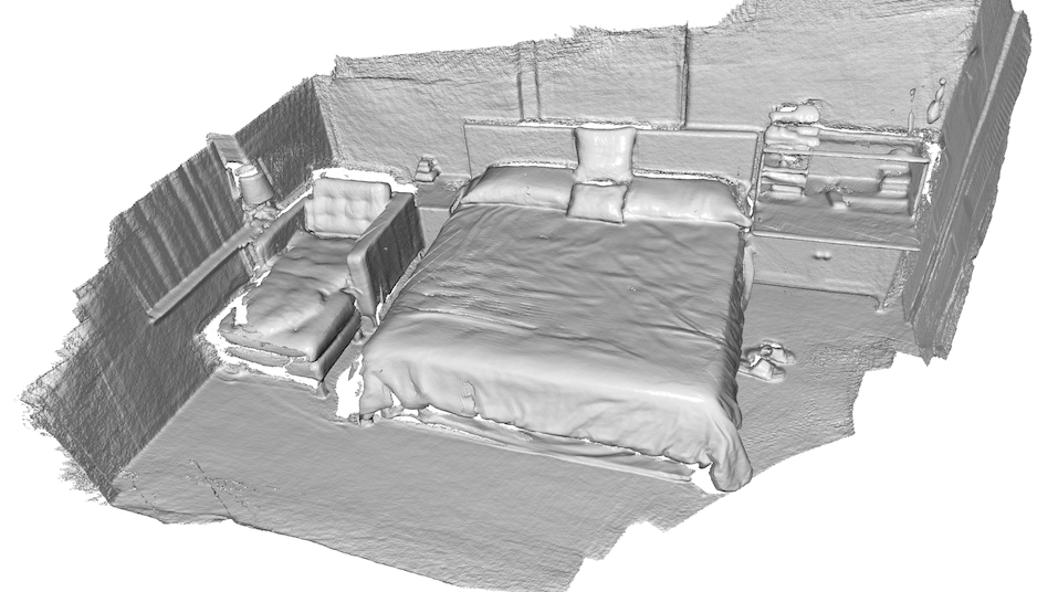
メッシュの抽出には Lorensen & amp; Cline(1987)のmarching cubesアルゴリズムを使用している。
Lorensen, W. E. & amp; H. E. Cline(1987) Marching cubes: A high resolution 3d surface construction algorithm, ACM Computer Graphics.
print("Extract a triangle mesh from the volume and visualize it.")
mesh = volume.extract_triangle_mesh()
mesh.compute_vertex_normals()
draw_geometries([mesh])
出力:h

# src/Python/Tutorial/Advanced/customized_visualization.py
%matplotlib inline

import os
from py3d import *
import numpy as np
import matplotlib.pyplot as plt

def custom_draw_geometry(pcd):
    # The following code achieves the same effect as:
    # draw_geometries([pcd])
    vis = Visualizer()
    vis.create_window()
    vis.add_geometry(pcd)
    vis.run()
    vis.destroy_window()

def custom_draw_geometry_with_rotation(pcd):
    def rotate_view(vis):
        ctr = vis.get_view_control()
        ctr.rotate(10.0, 0.0)
        return False
    draw_geometries_with_animation_callback([pcd], rotate_view)

def custom_draw_geometry_load_option(pcd):
    vis = Visualizer()
    vis.create_window()
    vis.add_geometry(pcd)
    vis.get_render_option().load_from_json(
            "./TestData/renderoption.json")
    vis.run()
    vis.destroy_window()

def custom_draw_geometry_with_key_callback(pcd):
    def change_background_to_black(vis):
        opt = vis.get_render_option()
        opt.background_color = np.asarray([0, 0, 0])
        return False
    def load_render_option(vis):
        vis.get_render_option().load_from_json(
                "./TestData/renderoption.json")
        return False
    def capture_depth(vis):
        depth = vis.capture_depth_float_buffer()
        plt.imshow(np.asarray(depth))
        plt.show()
        return False
    def capture_image(vis):
        image = vis.capture_screen_float_buffer()
        plt.imshow(np.asarray(image))
        plt.show()
        return False
    key_to_callback = {}
    key_to_callback[ord("K")] = change_background_to_black
    key_to_callback[ord("R")] = load_render_option
    key_to_callback[ord(",")] = capture_depth
    key_to_callback[ord(".")] = capture_image
    draw_geometries_with_key_callbacks([pcd], key_to_callback)

def custom_draw_geometry_with_camera_trajectory(pcd):
    custom_draw_geometry_with_camera_trajectory.index = -1
    custom_draw_geometry_with_camera_trajectory.trajectory =\
            read_pinhole_camera_trajectory(
                    "./TestData/camera_trajectory.json")
    custom_draw_geometry_with_camera_trajectory.vis = Visualizer()
    if not os.path.exists("./TestData/image/"):
        os.makedirs("./TestData/image/")
    if not os.path.exists("./TestData/depth/"):
        os.makedirs("./TestData/depth/")
    def move_forward(vis):
        # This function is called within the Visualizer::run() loop
        # The run loop calls the function, then re-render
        # So the sequence in this function is to:
        # 1. Capture frame
        # 2. index++, check ending criteria
        # 3. Set camera
        # 4. (Re-render)
        ctr = vis.get_view_control()
        glb = custom_draw_geometry_with_camera_trajectory
        if glb.index >= 0:
            print("Capture image {:05d}".format(glb.index))
            depth = vis.capture_depth_float_buffer(False)
            image = vis.capture_screen_float_buffer(False)
            plt.imsave("./TestData/depth/{:05d}.png".format(glb.index),\
                    np.asarray(depth), dpi = 1)
            plt.imsave("./TestData/image/{:05d}.png".format(glb.index),\
                    np.asarray(image), dpi = 1)
            #vis.capture_depth_image("depth/{:05d}.png".format(glb.index), False)
            #vis.capture_screen_image("image/{:05d}.png".format(glb.index), False)
        glb.index = glb.index + 1
        if glb.index < len(glb.trajectory.extrinsic):
            ctr.convert_from_pinhole_camera_parameters(glb.trajectory.intrinsic,\
                    glb.trajectory.extrinsic[glb.index])
        else:
            custom_draw_geometry_with_camera_trajectory.vis.\
                    register_animation_callback(None)
        return False
    vis = custom_draw_geometry_with_camera_trajectory.vis
    vis.create_window()
    vis.add_geometry(pcd)
    vis.get_render_option().load_from_json("./TestData/renderoption.json")
    vis.register_animation_callback(move_forward)
    vis.run()
    vis.destroy_window()

if __name__ == "__main__":
    pcd = read_point_cloud("./TestData/fragment.ply")

    print("1. Customized visualization to mimic DrawGeometry")
    custom_draw_geometry(pcd)

    print("2. Customized visualization with a rotating view")
    custom_draw_geometry_with_rotation(pcd)

    print("3. Customized visualization showing normal rendering")
    custom_draw_geometry_load_option(pcd)

    print("4. Customized visualization with key press callbacks")
    print("   Press 'K' to change background color to black")
    print("   Press 'R' to load a customized render option, showing normals")
    print("   Press ',' to capture the depth buffer and show it")
    print("   Press '.' to capture the screen and show it")
    custom_draw_geometry_with_key_callback(pcd)

    print("5. Customized visualization playing a camera trajectory")
    custom_draw_geometry_with_camera_trajectory(pcd)


Mimic draw_geometries() with Visualizer class
Visualizerクラスによるdraw_geometries()関数の模倣
def custom_draw_geometry(pcd):
    # The following code achieves the same effect as:
    # draw_geometries([pcd])
    vis = Visualizer()
    vis.create_window()
    vis.add_geometry(pcd)
    vis.run()
    vis.destroy_window()
この関数は、便利な関数draw_geometriesとまったく同じ機能を生成する。

クラスビジュアライザには、ViewControlやRenderOptionなどの変数がいくつかある。 次の関数は、jsonファイルに格納されている定義済みのRenderOptionを読み取るものである。
def custom_draw_geometry_load_option(pcd):
    vis = Visualizer()
    vis.create_window()
    vis.add_geometry(pcd)
    vis.get_render_option().load_from_json(
            "./TestData/renderoption.json")
    vis.run()
    vis.destroy_window()
出力:

Use callback functions
callback関数の使用
def custom_draw_geometry_with_rotation(pcd):
    def rotate_view(vis):
        ctr = vis.get_view_control()
        ctr.rotate(10.0, 0.0)
        return False
    draw_geometries_with_animation_callback([pcd], rotate_view)
関数draw_geometries_with_animation_callbackは、コールバック関数rotate_viewをメインループのアイドル関数として登録する。 ビジュアライザーがアイドル状態になると、x軸に沿ってビューが回転する。 これはつまりアニメーションの動作を定義しているのである。

def custom_draw_geometry_with_key_callback(pcd):
    def change_background_to_black(vis):
        opt = vis.get_render_option()
        opt.background_color = np.asarray([0, 0, 0])
        return False
    def load_render_option(vis):
        vis.get_render_option().load_from_json(
                "./TestData/renderoption.json")
        return False
    def capture_depth(vis):
        depth = vis.capture_depth_float_buffer()
        plt.imshow(np.asarray(depth))
        plt.show()
        return False
    def capture_image(vis):
        image = vis.capture_screen_float_buffer()
        plt.imshow(np.asarray(image))
        plt.show()
        return False
    key_to_callback = {}
    key_to_callback[ord("K")] = change_background_to_black
    key_to_callback[ord("R")] = load_render_option
    key_to_callback[ord(",")] = capture_depth
    key_to_callback[ord(".")] = capture_image
    draw_geometries_with_key_callbacks([pcd], key_to_callback)
コールバック機能は、キー・イベントに登録できる。 このスクリプトは4つのキーを登録している。 たとえば、Kを押すと背景色が黒に変わり、Rを押すとカスタム化したレンダーオプションを読み込み、,は深さ画像を.は画像をキャプチャする。以下はKを押したときの図

Capture images in a customized animation
カスタム化したアニメーションの画像のキャプチャ
def custom_draw_geometry_with_camera_trajectory(pcd):
    custom_draw_geometry_with_camera_trajectory.index = -1
    custom_draw_geometry_with_camera_trajectory.trajectory =\
            read_pinhole_camera_trajectory(
                    "./TestData/camera_trajectory.json")
    custom_draw_geometry_with_camera_trajectory.vis = Visualizer()
    if not os.path.exists("./TestData/image/"):
        os.makedirs("./TestData/image/")
    if not os.path.exists("./TestData/depth/"):
        os.makedirs("./TestData/depth/")
    def move_forward(vis):
        # This function is called within the Visualizer::run() loop
        # The run loop calls the function, then re-render
        # So the sequence in this function is to:
        # 1. Capture frame
        # 2. index++, check ending criteria
        # 3. Set camera
        # 4. (Re-render)
        ctr = vis.get_view_control()
        glb = custom_draw_geometry_with_camera_trajectory
        if glb.index >= 0:
            print("Capture image {:05d}".format(glb.index))
            depth = vis.capture_depth_float_buffer(False)
            image = vis.capture_screen_float_buffer(False)
            plt.imsave("./TestData/depth/{:05d}.png".format(glb.index),\
                    np.asarray(depth), dpi = 1)
            plt.imsave("./TestData/image/{:05d}.png".format(glb.index),\
                    np.asarray(image), dpi = 1)
            #vis.capture_depth_image("depth/{:05d}.png".format(glb.index), False)
            #vis.capture_screen_image("image/{:05d}.png".format(glb.index), False)
        glb.index = glb.index + 1
        if glb.index < len(glb.trajectory.extrinsic):
            ctr.convert_from_pinhole_camera_parameters(glb.trajectory.intrinsic,\
                    glb.trajectory.extrinsic[glb.index])
        else:
            custom_draw_geometry_with_camera_trajectory.vis.\
                    register_animation_callback(None)
        return False
    vis = custom_draw_geometry_with_camera_trajectory.vis
    vis.create_window()
    vis.add_geometry(pcd)
    vis.get_render_option().load_from_json("./TestData/renderoption.json")
    vis.register_animation_callback(move_forward)
    vis.run()
    vis.destroy_window()
この関数は、カメラの軌跡を読み込み、カメラの軌跡を移動するためにmove_forwardというアニメーション関数を定義している。 このアニメーション関数では、Visualizer.capture_depth_float_bufferとVisualizer.capture_screen_float_bufferをそれぞれ使用してカラー画像と深度画像の両方をキャプチャし、 それらをファイルに保存する。
取り込まれた画像シーケンス:

取り込まれた深さシーケンス:

Interactive visualization
対話的な可視化
このチュートリアルでは、ビジュアライザーウィンドウのユーザー対話機能を紹介する。
注: 次のコードではdemo_manual_registration関数の assert のところでエラーが起きるので外してある(2箇所)
# src/Python/Tutorial/Advanced/interactive_visualization.py

import numpy as np
import sys, copy
from py3d import *

def demo_crop_geometry():
    print("Demo for manual geometry cropping")
    print("1) Press 'Y' twice to align geometry with positive direction of y-axis")
    print("2) Press 'K' to lock screen and to switch to selection mode")
    print("3) Drag for rectangle selection,")
    print("   or use ctrl + left click for polygon selection")
    print("4) Press 'C' to get a selected geometry and to save it")
    print("5) Press 'F' to switch to freeview mode")
    pcd = read_point_cloud("./TestData/ICP/cloud_bin_0.pcd")
    draw_geometries_with_editing([pcd])

def draw_registration_result(source, target, transformation):
    source_temp = copy.deepcopy(source)
    target_temp = copy.deepcopy(target)
    source_temp.paint_uniform_color([1, 0.706, 0])
    target_temp.paint_uniform_color([0, 0.651, 0.929])
    source_temp.transform(transformation)
    draw_geometries([source_temp, target_temp])

def pick_points(pcd):
    print("")
    print("1) Please pick at least three correspondences using [shift + left click]")
    print("   Press [shift + right click] to undo point picking")
    print("2) Afther picking points, press q for close the window")
    vis = VisualizerWithEditing()
    vis.create_window()
    vis.add_geometry(pcd)
    vis.run() # user picks points
    vis.destroy_window()
    print("")
    return vis.get_picked_points()

def demo_manual_registration():
    print("Demo for manual ICP")
    source = read_point_cloud("./TestData/ICP/cloud_bin_0.pcd")
    target = read_point_cloud("./TestData/ICP/cloud_bin_2.pcd")
    print("Visualization of two point clouds before manual alignment")
    draw_registration_result(source, target, np.identity(4))

    # pick points from two point clouds and builds correspondences
    picked_id_source = pick_points(source)
    picked_id_target = pick_points(target)
    # assert(len(picked_id_source)>=3 and len(picked_id_target)>=3)
    # assert(len(picked_id_source) == len(picked_id_target))
    corr = np.zeros((len(picked_id_source),2))
    corr[:,0] = picked_id_source
    corr[:,1] = picked_id_target

    # estimate rough transformation using correspondences
    print("Compute a rough transform using the correspondences given by user")
    p2p = TransformationEstimationPointToPoint()
    trans_init = p2p.compute_transformation(source, target,
             Vector2iVector(corr))

    # point-to-point ICP for refinement
    print("Perform point-to-point ICP refinement")
    threshold = 0.03 # 3cm distance threshold
    reg_p2p = registration_icp(source, target, threshold, trans_init,
            TransformationEstimationPointToPoint())
    draw_registration_result(source, target, reg_p2p.transformation)
    print("")

if __name__ == "__main__":
    demo_crop_geometry()
    demo_manual_registration()
このスクリプトは、ユーザー対話の2つのアプリケーションdemo_crop_geometry()とdemo_manual_registration()を実行する。
Crop geometry
幾何形状の切り取り
def demo_crop_geometry():
    print("Demo for manual geometry cropping")
    print("1) Press 'Y' twice to align geometry with negative direction of y-axis")
    print("2) Press 'K' to lock screen and to switch to selection mode")
    print("3) Drag for rectangle selection,")
    print("   or use ctrl + left click for polygon selection")
    print("4) Press 'C' to get a selected geometry and to save it")
    print("5) Press 'F' to switch to freeview mode")
    pcd = read_point_cloud("./TestData/ICP/cloud_bin_0.pcd")
    draw_geometries_with_editing([pcd])
この関数はポイントクラウドを読み取り、draw_geometries_with_editingを呼び出す。 この関数は、頂点の選択とクロッピングを提供する。
注意:
Open3Dには、Visualizerクラスを継承するVisualizerWithEditingクラスがある。 これは、グラフィックユーザー対話機能を追加する。 カスタマイズされた視覚化の例と同様に、VisualizerWithEditing()をdraw_geometries_with_editing([pcd])の代わりに明示的に使用できる。
ジオメトリが表示されたら、Yを2回押してジオメトリをy軸の負の方向に揃える。 表示方向を調整したら、Kを押して画面をロックし、選択モードに切り替える。

demo_crop_geometry()
Tip 領域を選択するための実用的な方法は、正投影モデルを使用してジオメトリを任意の軸に揃えることである。 このトリックは、透視投影による自己閉塞の煩わしさを避けられるので、選択が容易になる。
領域を選択するには、マウスドラッグ(矩形選択)またはCtrl +左マウスクリック(ポリゴン選択)のいずれかを使用する。 以下の例は、ポリゴンを使用して選択した領域を示している。
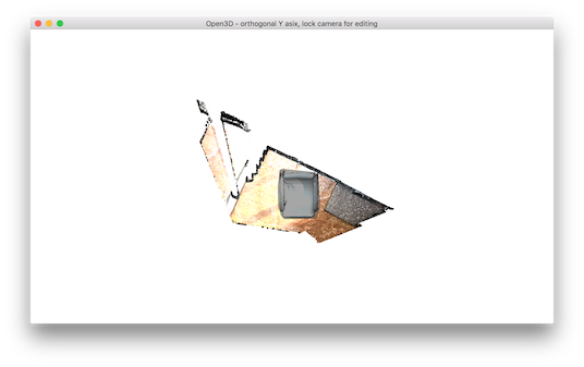
選択した領域は暗い影になっている。 選択した領域を保持し、残りの部分を破棄するには、Cを押す。するとトリミングされたジオメトリを保存するダイアログボックスが表示される。 そして保存後にクロッピング結果が表示される。
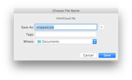

選択モードから抜けるにはFを押す。すると自由閲覧モードになる。
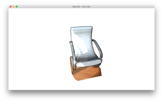
def demo_manual_registration():
    print("Demo for manual ICP")
    source = read_point_cloud("./TestData/ICP/cloud_bin_0.pcd")
    target = read_point_cloud("./TestData/ICP/cloud_bin_2.pcd")
    print("Visualization of two point clouds before manual alignment")
    draw_registration_result(source, target, np.identity(4))

    # pick points from two point clouds and builds correspondences
    picked_id_source = pick_points(source)
    picked_id_target = pick_points(target)
    (以下略)
このスクリプトは2つのポイントクラウドを読み取り、整列前にポイントクラウドを可視化する。

def pick_points(pcd):
    print("")
    print("1) Please pick at least three correspondences using [shift + left click]")
    print("   Press [shift + right click] to undo point picking")
    print("2) After picking points, press q for close the window")
    vis = VisualizerWithEditing()
    vis.create_window()
    vis.add_geometry(pcd)
    vis.run() # user picks points
    vis.destroy_window()
    print("")
    return vis.get_picked_points()
関数pick_points(pcd)は、VisualizerWithEditingのインスタンスを作成する。 draw_geometriesを模倣するために、ウィンドウを作成し、ジオメトリを追加し、ジオメトリを可視化し、終了する。 VisualizerWithEditinの新しいインタフェース関数は、ユーザが選択した頂点のインデックスを返すget_picked_points()である。
頂点を選択するには、ウィンドゥ上でShift + left クリックする。 頂点が選択されている場合、ビジュアライザーウィンドウは選択された頂点上の球をオーバーレイする。 たとえば、ソースのポイントクラウドで3つの頂点を選択したときは、次のように表示される。

pick_points(pcd)
qを押してウィンドウを閉じる。 次のステップは、ターゲットのポイントクラウドで同じ対応関係を選択することである。 球の色は同じ対応を識別するのに役立つ。

原文では
Picked point #58481 (2.14, 1.56, 1.53) to add in queue.
Picked point #77321 (2.86, 1.92, 1.09) to add in queue.
Picked point #42639 (3.28, 1.53, 1.45) to add in queue.
となると書いてあるが、原文のとおりには表示されない。少なくとも以下のようなコードが必要:
for p in pick_points(pcd):
    print("Picked point #%d %s to add in queue."%(p,str(pcd.points[p])))
Top 良い位置合わせ結果を得るには、シーン全体に分布するよう3つ以上のポイントを選ぶこと。特にコーナー領域に頂点を使用すると、適切な対応を簡単に選択することができる。
Registration using user correspondences
ユーザー指示の対応点を用いた位置合わせ
def demo_manual_registration():
    (前半省略、前からの続き)
    assert(len(picked_id_source)>=3 and len(picked_id_target)>=3)
    assert(len(picked_id_source) == len(picked_id_target))
    corr = np.zeros((len(picked_id_source),2))
    corr[:,0] = picked_id_source
    corr[:,1] = picked_id_target

    # estimate rough transformation using correspondences
    print("Compute a rough transform using the correspondences given by user")
    p2p = TransformationEstimationPointToPoint()
    trans_init = p2p.compute_transformation(source, target,
             Vector2iVector(corr))

    # point-to-point ICP for refinement
    print("Perform point-to-point ICP refinement")
    threshold = 0.03 # 3cm distance threshold
    reg_p2p = registration_icp(source, target, threshold, trans_init,
            TransformationEstimationPointToPoint())
    draw_registration_result(source, target, reg_p2p.transformation)
    print("")
デモの後半では、ユーザー提供の対応関係に基づいて初期変換を計算する。 このスクリプトは、Vector2iVector(corr)を使用して一対の対応を作成する。 これは、TransformationEstimationPointToPoint.compute_transformationを使用して、対応から初期変換を計算する。 最初の変換はregistration_icpを使用して精緻化される。
位置合わせ結果は次のとおり:

このチュートリアルでは、RGBDシーケンスから3Dシーンを再構成するための完全なパイプラインを示す。 パイプラインはChoi et al.(2015)に基づいている。 Park et al.(2017)で導入されたいくつかのアイデアは、より良い再現結果のために採用されている。
- Choi, S., Zhou, Q.-Y., & V. Koltun. (2015). Robust Reconstruction of Indoor Scenes, CVPR.
- Park, J., Zhou, Q.-Y., & V. Koltun (2017) Colored Point Cloud Registration Revisited, ICCV,
Example dataset
このチュートリアルでは、SceneNNデータセットを使用してシステムのデモンストレーションを行う。 これ以外に、Redwoodデータ、TUM RGBDデータ、ICL-NUIMデータ、SUN3Dデータなど、優れたRGBDデータセットを使うことができる。
このチュートリアルでは、SceneNNデータセットの016シーケンスを使用する。このシーケンスはSceneNN oni file archieveからのものである。 oniファイルは、Redwood再構成システムのOniParserを使用して、色と深さの画像シーケンスを抽出できる。これ以外に、.oniファイルを同期したRGBD画像のセットに変換するツールを使っても良いだろう。 このリンクは、016シーケンスをダウンロードするためのものである。
注: 以下をすすめるには、上記のリンクから016.oniファイルをダウンロードし、OniParserを用いて展開しておく必要がある
Quick start
すべてのカラー画像をImageフォルダに入れ、すべての深度画像をdepthフォルダに入れる。 ルートフォルダから次のコマンドを実行する。
cd <your_path_to_py3d_lib>/Tutorial/ReconstructionSystem/    # Open3D/build/lib/Tutorial/ReconstructionSystem のはず
python make_fragments.py [path_to_dataset] [-path_intrinsic (optional)]  # 以下path_to_datasetにはSceneNNデータセットへのパスを指定
python register_fragments.py [path_to_dataset]
python integrate_scene.py [path_to_dataset] [-path_intrinsic (optional)]