PCL/OpenNI tutorial 4: 3D object recognition (descriptors)¶
出典: http://robotica.unileon.es/index.php/PCL/OpenNI_tutorial_4:_3D_object_recognition_(descriptors))
ポイント・クラウド処理の最も興味深いアプリケーションの一つ、3D物体認識の基礎を学ぶことにしよう。 2Dにおける物体認識と同様、この技術は、クラウド内の優れたキーポイント(特徴点)を見つけ出し、以前に保存されたセットと照合することに基づくものである。 しかし3Dには2Dと比べいくつかの利点がある。それは、センサに対する物体の正確な位置と向きをかなりの精度で推定することができるということである。 また、3D物体認識は、クラッタ(後ろにある物体を前にある物体が隠しているような混雑状態のシーン)に対してより頑健な傾向がある。 最後に、物体形状に関する情報を持つことで、衝突回避や操作の把握に役立つ。
このチュートリアルでは、記述子の種類、PCLで使用できるタイプの数、およびそれらの計算方法について説明する。
概要¶
3D物体認識の基本は、探索対象の物体を含んでいるクラウドと別なクラウドとの間の対応関係を見つけることである。これを行うには、ポイントを曖昧さを伴うことなく比較する方法が必要である。今までは、XYZ座標、RGBカラーを格納するポイントを扱ってきましたが、これらの特徴のどれもが一意的なものではない。例えば連続スキャンにおいては異なる表面にあるポイントであっても同じ座標を共有できるし、カラー情報を使用すると2次元認識での問題、すなわち明るさの問題がでてきてしまう。
以前のチュートリアルでは、法線を紹介する前に特徴量について説明した。法線は、ポイントの近傍についての情報をコード化するため、特徴量の一つである。つまり、法線を計算するときに隣接点が考慮され、周囲の表面構造がどのようになっているかがわかる。しかしこれでは十分ではない。最適な特徴量は、次の基準を満たす必要がある。
- 変換に対する頑健さ:変換や回転などの剛体変換(ポイント間の距離を変えないもの)は、その特徴量に影響してはならない。クラウドを使っていても、違いがあってはいけない。
- ノイズに対する頑健さ。ノイズの原因となる測定誤差が、特徴量の推定を大きく変えてはならない。
- 解像度に対する不変性:異なる密度でサンプリングされた場合(ダウンサンプリングを行った後のように)、結果は同一または類似していなければならない。
ここに記述子が関係してくる。記述子とは、ポイントに対する複雑で正確なシグネチャであり、周囲の幾何形状に関する多くの情報をコード化したものである。記述子の目的は、ノイズ、解像度、変換によらず、複数のポイント・クラウドにわたってポイントを明確に識別することである。また中には、(姿勢が取得できる)視点のように、記述子が属すオブジェクトについての追加データを捉えたものもある。
 2個のクラウドのポイント間の対応を見つける
PCLには多くの3D記述子が実装されている。それぞれポイントに対して固有の値を計算する独自の方法がある。例えば、点の法線とその近傍の角度の差を使用するものや、ポイント間の距離を使用するものがある。このため、用途目的によっては本質的に有用であったり役立たずであったりする。ある記述子はスケール不変で、別の記述子はオブジェクトのオクルージョンに強いことがある。どのような記述子を選ぶかは、したいことによって決まる。
必要な値を計算した後、記述子のサイズを減らすための処理を実行する。結果はヒストグラムで表される。ヒストグラムを作成するために、記述子を構成する変数それぞれの値の範囲を$n$個に細分し、それぞれの発生数を数えあげる。例として1から100の範囲の値をとる変数を一個計算する記述子を考えてみよう。ビンを10個用意し、最初のビンは値が1から10の間にあるものの出現数を集め、2番目のビンは11から20までの出現数を集める、ということを繰り返す。例えばポイントの近傍点の変数の値が27であるとすれば、3番目のビンの値を1増加させる。このような操作を、そのキーポイントに対して最終的なヒストグラムが得られるまで続ける。ビンのサイズは、その変数をどのように記述するかに基づいて、慎重に選択する必要がある(どの変数に対しても同じ数のビンを用意する必要はなく、ビンも同じサイズである必要はない。例えばほとんどの値が50-100の範囲にあるとすれば、その範囲に対し、より小さなサイズのビンをたくさんもたせるのがよいだろう)。
記述子は、大局記述子と局所記述子というの2つに分類することができる。それぞれ計算して使用するプロセス(認識パイプライン)は異なるので、それぞれ別の節で説明する。
- Tutorials:
- Publication:
- Aitor Aldoma et al. (2012) Point Cloud Library: Three-Dimensional Object Recognition and 6 DoF Pose Estimation
| 名称 | 型 | サイズ† | カスタム ポイント型†† |
|---|---|---|---|
| SDSC (3D Shape Context) | 局所的 | 1980 | Yes |
| CVFH(Clustered Viewpoint Feature Histogram) | 大局的 | 308 | Yes |
| ESF(Ensemble of Shape Functions) | 大局的 | 640 | Yes |
| FPFH(Fast Point Feature Histogram) | 局所的 | 33 | Yes |
| GFPFH (Global Fast Point Feature Histogram) | 大局的 | 16 | Yes |
| GRSD (Global Radius-Based Surface Descriptor) | 大局的 | 21 | Yes |
| NARF (Normal Aligned Radial Feature) | 局所的 | 36 | Yes |
| OUR-CVFH (Oriented, Unique and Repeatable Clustered Viewpoint Feature Histogram) | 大局的 | 308 | Yes |
| PFH (Point Feature Histogram) | 局所的 | 125 | Yes |
| RIFT (Rotation-Invariant Feature Transform) | 局所的 | 32* | No |
| RoPS (Rotational Projection Statistics) | 局所的 | 135* | No |
| RSD (Radius-Based Surface Descriptor) | 局所的 | 289 | Yes |
| SHOT (Signatures of Histograms of Orientations) | 局所的 | 352 | Yes |
| Spin image | 局所的 | 153* | No |
| USC (Unique Shape Context) | 局所的 | 1960 | Yes |
| VFH (Viewpoint Feature Histogram) | 大局的 | 308 | Yes |
†アスタリスク(*)の付いた値は、記述子のサイズがいくつかのパラメータに依存することを示し、記載値はデフォルト値を示す。
††独自のカスタム・ポイント型を持たない記述子は、汎用の "pcl::Histogram <>"型を使用する。 保存と読み込みを参照せよ。
必要に応じて、単純なバージョンのテーブルでドキュメントをダウンロードすることも可能。 ページフォーマットはA4、ランドスケープである:
- Downloads:
- 元は ODTファイル (uses font embedding, requires LibreOffice 4)
- PDF形式の表
PFH¶
PFHとはPoint Feature Histogram(ポイント特徴量ヒストグラム)の略である。これは、PCLによって提供される最も重要な記述子の1つであり、FPFHなどの他のものの基礎にもなっている。 PFHは、近傍の法線の方向の違いを分析することにより、点を取り囲む幾何形状の情報を捉えようとする(このため、不正確な法線推定は質の低い記述子を生成する可能性がある)。
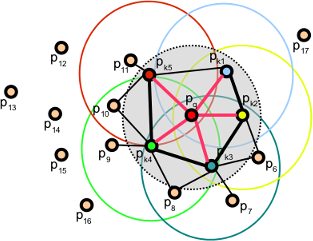
第1に、このアルゴリズムは、すべての近傍点同士のペアを作る(選択したキーポイントと近傍点とのペアだけでなく、近傍点同士のペアも作る)。次に、ペアそれぞれに対して、その法線から固定座標フレームを計算する。このフレームにより、法線の差異を3つの角度変数で符号化できる。この変数は、点間のユークリッド距離とともに記憶され、すべてのペアに対する計算結果からヒストグラムが作られる。最終的な記述子は、各変数(合計4つ)のヒストグラムの連結である。


(左)ポイントのPFH計算に設定されるポイント・ペア
(右)ペアの1つに対し計算された固定座標フレームと角度特徴量
PCLでは、記述子の計算は非常に簡単で、PFHも例外ではない。
#include <pcl/io/pcd_io.h>
#include <pcl/features/normal_3d.h>
#include <pcl/features/pfh.h>

int
main(int argc, char** argv)
{
	// Object for storing the point cloud.   ポイントクラウドの格納用オブジェクト
	pcl::PointCloud<pcl::PointXYZ>::Ptr cloud(new pcl::PointCloud<pcl::PointXYZ>);
	// Object for storing the normals.      法線の格納用オブジェクト
	pcl::PointCloud<pcl::Normal>::Ptr normals(new pcl::PointCloud<pcl::Normal>);
	// Object for storing the PFH descriptors for each point.  それぞれのポイントに対するPFH記述子の格納用オブジェクト
	pcl::PointCloud<pcl::PFHSignature125>::Ptr descriptors(new pcl::PointCloud<pcl::PFHSignature125>());

	// Read a PCD file from disk.    ハードディスクからPCDファイルを読み込む
	if (pcl::io::loadPCDFile<pcl::PointXYZ>(argv[1], *cloud) != 0)
	{
		return -1;
	}

	// Note: you would usually perform downsampling now. It has been omitted here
	// for simplicity, but be aware that computation can take a long time.
    // 注意: 普通はここでダウンサンプリングを行う。このコードでは省略しているが、時間がかかることに注意

	// Estimate the normals.   法線の推定
	pcl::NormalEstimation<pcl::PointXYZ, pcl::Normal> normalEstimation;
	normalEstimation.setInputCloud(cloud);
	normalEstimation.setRadiusSearch(0.03);
	pcl::search::KdTree<pcl::PointXYZ>::Ptr kdtree(new pcl::search::KdTree<pcl::PointXYZ>);
	normalEstimation.setSearchMethod(kdtree);
	normalEstimation.compute(*normals);

	// PFH estimation object.     PFH推定のためのオブジェクト
	pcl::PFHEstimation<pcl::PointXYZ, pcl::Normal, pcl::PFHSignature125> pfh;
	pfh.setInputCloud(cloud);
	pfh.setInputNormals(normals);
	pfh.setSearchMethod(kdtree);
	// Search radius, to look for neighbors. Note: the value given here has to be
	// larger than the radius used to estimate the normals.
    // 近接点を探すための探索半径。注意: ここでの値は法線推定のため半径よりも大きくなければならない
	pfh.setRadiusSearch(0.05);

	pfh.compute(*descriptors);
}
見てのとおり、PCLは "PFHSignature125"タイプを使用して記述子を保存する。これは、記述子のサイズが125(特徴ベクトルの次元数)であることを意味する。 $D$次元の特徴量を次元ごとに$B$個に分割するには、合計$B^D$個のビンが必要である。元々の提案は3つの角度特徴量以外にポイント間の距離を利用していたが、PCLの実装では距離は使っていない、というのは(特にセンサから離れるほどポイント間の距離が増える2.5Dスキャンでは)十分な分離性能をもたないためである。したがって、残りの特徴量(それぞれ1次元)は5分割され、合計125次元($5^3$)のベクトルとなる。
計算結果の記述子を格納する最終的なオブジェクトは、普通のクラウド(ハードディスクに保存されていても)のように扱うことができ、元のクラウドと同じ数の「ポイント」を持つ。たとえば、位置0の「PFHSignature125」オブジェクトは、クラウドの同じ位置の「PointXYZ」ポイントに対するPFH記述子を格納している。
記述子の詳細については、以下の出版物やPCLのチュートリアルを参照のこと。
- 入力: ポイント、法線、探索手法、半径
- 出力: PFH 記述子
- Tutorial: Point Feature Histograms (PFH) descriptors (参考)
- Publications:
- Radu Bogdan Rusu et al. (2008) Persistent Point Feature Histograms for 3D Point Clouds
- Radu Bogdan Rusu (2009) Semantic 3D Object Maps for Everyday Manipulation in Human Living Environments section 4.4, p. 50.
- API: pcl::PFHEstimation
- Download
FPFH¶
FHでは正確な結果が得られるが、リアルタイムで実行するには計算コストがかかりすぎる欠点がある。 $k$個の近傍を考慮した$n$個のキーポイントのクラウドの場合、$O(nk^2)$の計複が要求される。 このため、FPFH(Fast Point Feature Histogram、高速ポイント特徴量ヒストグラム)という名前の派生記述子が作成された。
FPFHは、現在のキーポイントとその近接点間の直接接続のみを考慮し、近接点間の追加リンクを削除する。 これにより計算の複雑さを$O(nk)$まで減らす。 このため、結果のヒストグラムはSPFH(Simplified Point Feature Histogram)と呼ばれる。 参照フレーム(基準座標系)と角度変数はいつもどおり計算される。
 ポイントのFPFHを計算するときに設定されるポイント対
追加リンクを削除したことを補うために、すべてのヒストグラムを計算した後で追加ステップを実行する、つまりポイントの近隣のSPFHが距離に応じて重み付けしたものを「マージ」する。 これは、使用される半径の2倍の距離にある点の情報を与えるという効果がある。 最後に、3つのヒストグラム(距離は使用しない)を連結して最終的な記述子を構成する。
#include <pcl/io/pcd_io.h>
#include <pcl/features/normal_3d.h>
#include <pcl/features/fpfh.h>

int
main(int argc, char** argv)
{
	// Object for storing the point cloud.  ポイントクラウドの格納用オブジェクト
	pcl::PointCloud<pcl::PointXYZ>::Ptr cloud(new pcl::PointCloud<pcl::PointXYZ>);
	// Object for storing the normals.    法線の格納用オブジェクト
	pcl::PointCloud<pcl::Normal>::Ptr normals(new pcl::PointCloud<pcl::Normal>);
	// Object for storing the FPFH descriptors for each point. それぞれのポイントに対するFPFH記述子の格納用オブジェクト
	pcl::PointCloud<pcl::FPFHSignature33>::Ptr descriptors(new pcl::PointCloud<pcl::FPFHSignature33>());

	// Read a PCD file from disk.  ハードディスクからPCDファイルを読み込む
	if (pcl::io::loadPCDFile<pcl::PointXYZ>(argv[1], *cloud) != 0)
	{
		return -1;
	}

	// Note: you would usually perform downsampling now. It has been omitted here
	// for simplicity, but be aware that computation can take a long time.
    // 注意: 普通はここでダウンサンプリングを行う。このコードでは省略しているが、時間がかかることに注意

	// Estimate the normals. 法線の推定
	pcl::NormalEstimation<pcl::PointXYZ, pcl::Normal> normalEstimation;
	normalEstimation.setInputCloud(cloud);
	normalEstimation.setRadiusSearch(0.03);
	pcl::search::KdTree<pcl::PointXYZ>::Ptr kdtree(new pcl::search::KdTree<pcl::PointXYZ>);
	normalEstimation.setSearchMethod(kdtree);
	normalEstimation.compute(*normals);

	// FPFH estimation object.   FPFH推定のためのオブジェクト
	pcl::FPFHEstimation<pcl::PointXYZ, pcl::Normal, pcl::FPFHSignature33> fpfh;
	fpfh.setInputCloud(cloud);
	fpfh.setInputNormals(normals);
	fpfh.setSearchMethod(kdtree);
	// Search radius, to look for neighbors. Note: the value given here has to be
	// larger than the radius used to estimate the normals.
    // 近接点を探すための探索半径。注意: ここでの値は法線推定のため半径よりも大きくなければならない
	fpfh.setRadiusSearch(0.05);

	fpfh.compute(*descriptors);
}
マルチスレッド最適化(OpenMP APIを使用)を利用するFPFH推定の追加実装は、クラス "FPFHEstimationOMP"で使用できる。 そのインタフェースは、標準的な非最適化版の実装と同じである。 これを用いると、マルチコア・システムにおいてパフォーマンスが大幅に向上し、計算時間が短縮される。ただしヘッダーファイル「fpfh_omp.h」をincludeすることを忘れないように。
- 入力:ポイント、法線、探索手法、半径
- 出力: FPFH 記述子
- Tutorial: Fast Point Feature Histograms (FPFH) descriptors (参考)
- Publications:
- Radu Bogdan Rusu et al.(2009) Fast Point Feature Histograms (FPFH) for 3D Registration
- Radu Bogdan Rusu, (2009) Semantic 3D Object Maps for Everyday Manipulation in Human Living Environments, Section 4.5, page 57.
- API:
- Download
RSD¶
RSD (Radius-Based Surface Descriptor, 半径系表面記述子)は、ポイントとその近傍の半径方向の関係をコード化する。 キーポイントと近傍点とのすべてのペアに対し、このアルゴリズムはそれらの間の距離と法線の差を計算する。 次に、両方の点がともに同じ球の表面上にあると仮定し、2つの点と法線に合う球を求める(そうでないと無限の可能な球が存在する)。 最後に、点の近傍点との球すべてから、最大半径と最小半径を持つものだけを記憶し、その点の記述子として記録する。
推測されるように、2つの点が平面上にあるときは球の半径は無限になる。 一方、それらが円筒の湾曲面上にある場合は、級の半径は円筒の半径とほぼ同じである。 これにより、RSDにより物体を識別することができる。このアルゴリズムのパラメータは、点の集まりを平面の一部とみなせるための最大半径である。


(左)法線を持つ2個のポイントに適合する球面
(右)クラウドのRSD値;平面上のポイントは最大値を持つ
画像の出典: http://ias.in.tum.de/_media/events/rgbd2011/marton.pdf
次はRSD記述子の計算のためのコードである:
#include <pcl/io/pcd_io.h>
#include <pcl/features/normal_3d.h>
#include <pcl/features/rsd.h>

int
main(int argc, char** argv)
{
	// Object for storing the point cloud.  ポイントクラウドの格納用オブジェクト
	pcl::PointCloud<pcl::PointXYZ>::Ptr cloud(new pcl::PointCloud<pcl::PointXYZ>);
	// Object for storing the normals.    法線の格納用オブジェクト
	pcl::PointCloud<pcl::Normal>::Ptr normals(new pcl::PointCloud<pcl::Normal>);
	// Object for storing the RSD descriptors for each point. 各ポイントに対するRSD記述子の格納用オブジェクト
	pcl::PointCloud<pcl::PrincipalRadiiRSD>::Ptr descriptors(new pcl::PointCloud<pcl::PrincipalRadiiRSD>());

	// Read a PCD file from disk.  ハードディスクからPCDファイルを読み込む
	if (pcl::io::loadPCDFile<pcl::PointXYZ>(argv[1], *cloud) != 0)
	{
		return -1;
	}

	// Note: you would usually perform downsampling now. It has been omitted here
	// for simplicity, but be aware that computation can take a long time.
    // 注意: 普通はここでダウンサンプリングを行う。このコードでは省略しているが、時間がかかることに注意

	// Estimate the normals.       法線の推定
	pcl::NormalEstimation<pcl::PointXYZ, pcl::Normal> normalEstimation;
	normalEstimation.setInputCloud(cloud);
	normalEstimation.setRadiusSearch(0.03);
	pcl::search::KdTree<pcl::PointXYZ>::Ptr kdtree(new pcl::search::KdTree<pcl::PointXYZ>);
	normalEstimation.setSearchMethod(kdtree);
	normalEstimation.compute(*normals);

	// RSD estimation object.     RSD推定のためのオブジェクト
	pcl::RSDEstimation<pcl::PointXYZ, pcl::Normal, pcl::PrincipalRadiiRSD> rsd;
	rsd.setInputCloud(cloud);
	rsd.setInputNormals(normals);
	rsd.setSearchMethod(kdtree);
	// Search radius, to look for neighbors. Note: the value given here has to be
	// larger than the radius used to estimate the normals.
	rsd.setRadiusSearch(0.05);
	// Plane radius. Any radius larger than this is considered infinite (a plane).
    // 平面半径。これより大きな半径はみな無限大(つまり平面)とみなされる
	rsd.setPlaneRadius(0.1);
	// Do we want to save the full distance-angle histograms?
    // 完全距離-角度ヒストグラムを格納したいか? false --- 格納しない
	rsd.setSaveHistograms(false);

	rsd.compute(*descriptors);
}
注:このコードはPCLバージョン1.8以上(現在のバージョン)でのみコンパイルできる。
必要に応じて、 "setSaveHistograms()"関数を用いて完全な距離-角度ヒストグラムを保存し、 "getHistograms()"を用いてこれを復元できる。
- 入力: ポイント、法線、探索手法、半径、最大半径、(分割), (完全ヒストグラム保存)
- 出力: RSD 記述子
- Publications:
- Zoltan-Csaba Marton et al. (2010) General 3D Modelling of Novel Objects from a Single View
- Zoltan-Csaba Marton et al. (2011) Combined 2D-3D Categorization and Classification for Multimodal Perception Systems
- API: pcl::RSDEstimation
- Download
3DSC¶
3D Shape Context(3次元形状コンテキスト)は、既にある2次元用の記述子を3次元に拡張したものである。 これは、指定された検索半径でディスクリプタを計算しているポイントを中心とするサポート構造(正確には球)を作成する。 その球の「北極」(「上」の概念)は、そのポイントの法線に一致するように設定する。 次に球を3D領域の区画、つまりビンに分割する。 最初の2つの座標(方位角と仰角)は、等間隔に分割する、3つ目(半径長さの次元)では分割を対数的に行い、球の中心に向かって小さくとる。ビンが小さくなり過ぎないよう最小半径を指定することができる。これは、表面形状における小さな変化に敏感すぎるからである。
ポイントに対する3DSCを計算するためのサポート構造(球)
ビンそれぞれに対し、ビン内の近接点すべてに重み付けして総和をとる。この重みはビンの体積と局所的な点の密度(現在の近接点周辺の点の個数)によって決まる。これにより、記述子はある程度の解像度不変性が与えられる。
サポート球には法線方向が与えられていると述べた。これにより自由度が一つ与えられる(2軸だけが固定されており、方位角は自由のままである)。そのため、ここまで述べてきた記述子は回転に対応していない。 これを克服するために(異なる2つのクラウドにおいて同じポイントが同じ値を持つようにするため)、サポート球を法線周りにN回(Nは方位角の分割に対応する度数)回転させ、 そのポイントに対し合計N個の記述子を作り出す処理を施す。
3DSC記述子は、次のように計算できる。
#include <pcl/io/pcd_io.h>
#include <pcl/features/normal_3d.h>
#include <pcl/features/3dsc.h>

int
main(int argc, char** argv)
{
	// Object for storing the point cloud. ポイントクラウドの格納用オブジェクト
	pcl::PointCloud<pcl::PointXYZ>::Ptr cloud(new pcl::PointCloud<pcl::PointXYZ>);
	// Object for storing the normals. 法線の格納用オブジェクト
	pcl::PointCloud<pcl::Normal>::Ptr normals(new pcl::PointCloud<pcl::Normal>);
	// Object for storing the 3DSC descriptors for each point. それぞれのポイントに対する3DSC記述子の格納用オブジェクト
	pcl::PointCloud<pcl::ShapeContext1980>::Ptr descriptors(new pcl::PointCloud<pcl::ShapeContext1980>());

	// Read a PCD file from disk. ハードディスクからPCDファイルを読み込む
	if (pcl::io::loadPCDFile<pcl::PointXYZ>(argv[1], *cloud) != 0)
	{
		return -1;
	}

	// Note: you would usually perform downsampling now. It has been omitted here
	// for simplicity, but be aware that computation can take a long time.
    // 注意: 普通はここでダウンサンプリングを行う。このコードでは省略しているが、時間がかかることに注意

	// Estimate the normals. 法線の推定
	pcl::NormalEstimation<pcl::PointXYZ, pcl::Normal> normalEstimation;
	normalEstimation.setInputCloud(cloud);
	normalEstimation.setRadiusSearch(0.03);
	pcl::search::KdTree<pcl::PointXYZ>::Ptr kdtree(new pcl::search::KdTree<pcl::PointXYZ>);
	normalEstimation.setSearchMethod(kdtree);
	normalEstimation.compute(*normals);

	// 3DSC estimation object. 3DSC推定のためのオブジェクト
	pcl::ShapeContext3DEstimation<pcl::PointXYZ, pcl::Normal, pcl::ShapeContext1980> sc3d;
	sc3d.setInputCloud(cloud);
	sc3d.setInputNormals(normals);
	sc3d.setSearchMethod(kdtree);
	// Search radius, to look for neighbors. It will also be the radius of the support sphere.
    // 近接点を探すための探索半径。サポート球の半径でもある
	sc3d.setRadiusSearch(0.05);
	// The minimal radius value for the search sphere, to avoid being too sensitive
	// in bins close to the center of the sphere.
    // 探索球のための最小半径、ビンが球の中心に近い時に微小変化に敏感になりすぎないようにするためのもの
	sc3d.setMinimalRadius(0.05 / 10.0);
	// Radius used to compute the local point density for the neighbors
	// (the density is the number of points within that radius).
    // 近接点に対し、局所点密度の計算に用いられる半径(密度とはその半径の中の点の個数)
	sc3d.setPointDensityRadius(0.05 / 5.0);

	sc3d.compute(*descriptors);    // 3DSCの計算、descriptorsに記述子が格納される
}
- 入力: ポイント、法線、探索手法、半径、ポイント密度半径
- 出力: 3DSC記述子
- Publication:
- Andrea Frome et al. (2004). Recognizing Objects in Range Data Using Regional Point Descriptors
- API: pcl::ShapeContext3DEstimation
- Download
USC¶
Unique Shape Context descriptor(USD, 一意的形状コンテキスト記述子)は、各ポイントに一意的な方向を与えるために、局所参照座標系(LRF, local reference frame)を定義することにより3DSCを拡張したものである。 これは、記述子の精度を向上させるだけでなく、向きを考慮した複数の記述子を計算する必要がなくなるため、記述子のサイズも小さくなる。
局所参照座標系(LRF)の計算方法の詳細については、下記の2番めの論文を参照のこと。
#include <pcl/io/pcd_io.h>
#include <pcl/features/usc.h>

int
main(int argc, char** argv)
{
	// Object for storing the point cloud. ポイントクラウドの格納用オブジェクト
	pcl::PointCloud<pcl::PointXYZ>::Ptr cloud(new pcl::PointCloud<pcl::PointXYZ>);
	// Object for storing the USC descriptors for each point. それぞれのポイントに対するUSC記述子の格納用オブジェクト
	pcl::PointCloud<pcl::UniqueShapeContext1960>::Ptr descriptors(new pcl::PointCloud<pcl::UniqueShapeContext1960>());

	// Read a PCD file from disk. ハードディスクからPCDファイルを読み込
	if (pcl::io::loadPCDFile<pcl::PointXYZ>(argv[1], *cloud) != 0)
	{
		return -1;
	}

	// Note: you would usually perform downsampling now. It has been omitted here
	// for simplicity, but be aware that computation can take a long time.
    // 注意: 普通はここでダウンサンプリングを行う。このコードでは省略しているが、時間がかかることに注意

	// USC estimation object.  USC推定オブジェクト
	pcl::UniqueShapeContext<pcl::PointXYZ, pcl::UniqueShapeContext1960, pcl::ReferenceFrame> usc;
	usc.setInputCloud(cloud);
	// Search radius, to look for neighbors. It will also be the radius of the support sphere.
    // 近接点を探すための探索半径。サポート球の半径でもある
	usc.setRadiusSearch(0.05);
	// The minimal radius value for the search sphere, to avoid being too sensitive
	// in bins close to the center of the sphere.
    // 探索球のための最小半径、ビンが球の中心に近い時に微小変化に敏感になりすぎないようにするためのもの
	usc.setMinimalRadius(0.05 / 10.0);
	// Radius used to compute the local point density for the neighbors
	// (the density is the number of points within that radius).
    // 近接点に対し、局所点密度の計算に用いられる半径(密度とはその半径の中の点の個数)
	usc.setPointDensityRadius(0.05 / 5.0);
	// Set the radius to compute the Local Reference Frame. 局所参照座標系を計算するための半径の設定
	usc.setLocalRadius(0.05);

	usc.compute(*descriptors);
}
注:このコードはPCLバージョン1.8以上(現在のバージョン)でのみコンパイルできる。 1.7以下の場合は、UniqueShapeContext1960をShapeContext1980に変更し、CMakeLists.txtを編集すること。
- 入力: ポイント、半径、最小半径、ポイント密度半径、局所半径
- 出力: USC 記述子
- Publication:
- Federico Tombari et al. (2010) Unique Shape Context for 3D Data Description
- Federico Tombari et al. (2010) Unique Signatures of Histograms for Local Surface Description
- API: pcl::UniqueShapeContext
- Download
SHOT¶
SHOTとはSignature of Histograms of Orientations(方向ヒストグラムのシグネチャ)の省略形である。3DSCと同様に、球形のサポート構造内のトポロジ(表面)についての情報を符号化している。この球体は、32のビン、つまり部分領域で分割され、方位角に沿って8つの区画、仰角に沿って2つ、半径に沿って2つの区画がある。どの部分領域(ビン)に対しても、1次元の局所ヒストグラムが計算される。ここでの変数は、キーポイントの法線とそのサポート構造内の点との間の角度(正確には余弦、とした方が適切ということが判明している)である。

SHOTの計算のためのサポート構造。明瞭化のために方位角にそって4分割しか示していない
すべての局所ヒストグラムが計算されると、最終的な記述子としてひとまとめにされる。 USC記述子と同様に、SHOTは局所参照座標系を使用して回転不変にする。 ノイズやクラッタ(後ろにある物体を前にある物体が隠しているような混雑状態のシーン)に対しても頑健である。
#include <pcl/io/pcd_io.h>
#include <pcl/features/normal_3d.h>
#include <pcl/features/shot.h>

int
main(int argc, char** argv)
{
	// Object for storing the point cloud.  ポイントクラウドの格納用オブジェクト
	pcl::PointCloud<pcl::PointXYZ>::Ptr cloud(new pcl::PointCloud<pcl::PointXYZ>);
	// Object for storing the normals.    法線の格納用オブジェクト
	pcl::PointCloud<pcl::Normal>::Ptr normals(new pcl::PointCloud<pcl::Normal>);
	// Object for storing the SHOT descriptors for each point. それぞれのポイントに対するSHOT記述子の格納用オブジェクト
	pcl::PointCloud<pcl::SHOT352>::Ptr descriptors(new pcl::PointCloud<pcl::SHOT352>());

	// Read a PCD file from disk.  ハードディスクからPCDファイルを読み込む
	if (pcl::io::loadPCDFile<pcl::PointXYZ>(argv[1], *cloud) != 0)
	{
		return -1;
	}

	// Note: you would usually perform downsampling now. It has been omitted here
	// for simplicity, but be aware that computation can take a long time.
    // 注意: 普通はここでダウンサンプリングを行う。このコードでは省略しているが、時間がかかることに注意

	// Estimate the normals.   法線の推定
	pcl::NormalEstimation<pcl::PointXYZ, pcl::Normal> normalEstimation;
	normalEstimation.setInputCloud(cloud);
	normalEstimation.setRadiusSearch(0.03);
	pcl::search::KdTree<pcl::PointXYZ>::Ptr kdtree(new pcl::search::KdTree<pcl::PointXYZ>);
	normalEstimation.setSearchMethod(kdtree);
	normalEstimation.compute(*normals);

	// SHOT estimation object.    SHOT推定のためのオブジェクト
	pcl::SHOTEstimation<pcl::PointXYZ, pcl::Normal, pcl::SHOT352> shot;
	shot.setInputCloud(cloud);
	shot.setInputNormals(normals);
	// The radius that defines which of the keypoint's neighbors are described.
	// If too large, there may be clutter, and if too small, not enough points may be found.
    // キーポイントの近傍点決定のための半径、大きすぎるとクラッタがおこりやすく、小さすぎると近傍点数が少なくなりすぎる
	shot.setRadiusSearch(0.02);

	shot.compute(*descriptors);
}
FPFHと同様に、OpenMPを利用する "SHOTEstimationOMP"を使用して、マルチスレッドに最適化されたものを利用できる。それにはヘッダーファイル "shot_omp.h"を含める必要がある。 また、マッチングのためにテクスチャを使用する別のバリエーション "SHOTColorEstimation"も用意されている(詳細については、下記の2番めの論文を参照すること)。 出力は"SHOT1344"記述子である。
- 入力: ポイント、法線、半径
- 出力: SHOT 記述子
- Publications:
- Federico Tombari et al. (2010) Unique Signatures of Histograms for Local Surface Description
- Federico Tombari et al. (2011) A Combined Texture-Shaped Descriptor for Enhanced 3D Feature Matching
- API:
- Download
Spin image¶
SpinImage(SI, スピンイメージ)はこの中で最も古い記述子である。 1997年から使われており、今でも特定の用途にはまだ使用されている。 もともとは、頂点、エッジ、ポリゴンによって作成された表面を記述するために設計されたものであるが、ポイントクラウドにも適用されている。 この記述子は他の記述しと異なり、出力がイメージ(画像)と似ており、通常の手段で比較できるものである。
用いられるサポート構造は、所定の半径および高さを有し、ある点を中心として、法線と位置合わせされた円筒である。 この円筒は、半径方向および垂直方向に領域分割される。 それぞれの領域ごとに、内部にある隣接点の数が合計され、最終的に記述子が作られる。結果の改善のために、重み付けと補間が用いられる。 最終的な記述子は、点密度が濃い領域が黒く表示される白黒画像として見ることができる。

モデルの3点に対し計算されたスピンイメージ
#include <pcl/io/pcd_io.h>
#include <pcl/features/normal_3d.h>
#include <pcl/features/spin_image.h>

// A handy typedef.  便利な構造体定義
typedef pcl::Histogram<153> SpinImage;

int
main(int argc, char** argv)
{
	// Object for storing the point cloud. ポイントクラウドの記憶用オブジェクト
	pcl::PointCloud<pcl::PointXYZ>::Ptr cloud(new pcl::PointCloud<pcl::PointXYZ>);
	// Object for storing the normals.  法線記憶用オブジェクト
	pcl::PointCloud<pcl::Normal>::Ptr normals(new pcl::PointCloud<pcl::Normal>);
	// Object for storing the spin image for each point.
    // 各ポイントについてのスピンイメージを記憶用のオブジェクト
	pcl::PointCloud<SpinImage>::Ptr descriptors(new pcl::PointCloud<SpinImage>());

	// Read a PCD file from disk.  PCDファイルをハードディスクから読み込む
	if (pcl::io::loadPCDFile<pcl::PointXYZ>(argv[1], *cloud) != 0)
	{
		return -1;
	}

	// Note: you would usually perform downsampling now. It has been omitted here
	// for simplicity, but be aware that computation can take a long time.
    // 注意: 普通はここでダウンサンプリングを行う。このコードでは省略しているが、時間がかかることに注意

	// Estimate the normals.   法線の推定
	pcl::NormalEstimation<pcl::PointXYZ, pcl::Normal> normalEstimation;
	normalEstimation.setInputCloud(cloud);
	normalEstimation.setRadiusSearch(0.03);
	pcl::search::KdTree<pcl::PointXYZ>::Ptr kdtree(new pcl::search::KdTree<pcl::PointXYZ>);
	normalEstimation.setSearchMethod(kdtree);
	normalEstimation.compute(*normals);

	// Spin image estimation object. スピンイメージ推定オブジェクト
	pcl::SpinImageEstimation<pcl::PointXYZ, pcl::Normal, SpinImage> si;
	si.setInputCloud(cloud);
	si.setInputNormals(normals);
	// Radius of the support cylinder.  サポート円筒の半径
	si.setRadiusSearch(0.02);
	// Set the resolution of the spin image (the number of bins along one dimension).
	// Note: you must change the output histogram size to reflect this.
    // スピンイメージの解像度(ひとつの次元に沿ったビンの個数)の設定
    // 注意: これを反映させるには出力ヒストグラムの変更が必要
	si.setImageWidth(8);

	si.compute(*descriptors);
}
スピンイメージ推定オブジェクトは、推定をチューニングするためいろいろな方法を提供しているので、APIを調べておくことが推奨される。
- 入力: ポイント、法線、半径、画像の解像度
- 出力: スピンイメージ
- Publications:
- Andrew Edie Johnson (1997) Spin-Images: A Representation for 3-D Surface Matching
- Andrew Edie Johnson & Martial Hebert (1999) Using Spin Images for Efficient Object Recognition in Cluttered 3D Scenes
- API: pcl::SpinImageEstimation
- Download
RIFT¶
Rotation-Invariant Feature Transform (RIFT, 回転不変特徴変換)は、スピンイメージと同様、2D特徴量のアイデア、つまりScale-Invariant Feature Transform(SIFT、スケール不変特徴変換)を用いたものである。 そのため輝度情報(RGB色値から取得できる)を必要とし、そのような記述子はここでとりあげる記述子の中では唯一のものである。もちろんこのことは、標準のXYZクラウドではRIFTを使用することができないことを意味する。テクスチャ情報も必要なのである。
最初のステップでは、注目点がある表面に(所定の半径を持つ)円形のパッチを当てはめる。 このパッチは、選んだ距離ビンのサイズに応じて同心円に分割される。 次に、その点を中心とし、上記の半径を持つ球の内側にあるすべての点の近傍点によりヒストグラムが作られる。 各点における強度勾配の方向と距離とが考慮される。 回転不変にするために、パッチの中心から外側に向くベクトルと強度勾配方向との角度を測定する。

記述子内の3つの異なる位置のRIFT特徴量
オリジナルの実装では、4つの同心円と8つの勾配ヒストグラムが用いられていたので記述子のサイズは32であった。RIFTはテクスチャの反転に強くないが、これは大きな問題とはみなされていなかった。
#include <pcl/io/pcd_io.h>
#include <pcl/point_types_conversion.h>
#include <pcl/features/normal_3d.h>
#include <pcl/features/intensity_gradient.h>
#include <pcl/features/rift.h>

// A handy typedef.
typedef pcl::Histogram<32> RIFT32;

int
main(int argc, char** argv)
{
	// Object for storing the point cloud with color information.
    // 色情報付きポイントクラウドを格納するためのオブジェクト
	pcl::PointCloud<pcl::PointXYZRGB>::Ptr cloudColor(new pcl::PointCloud<pcl::PointXYZRGB>);
	// Object for storing the point cloud with intensity value.
    // 輝度値をもつポイントクラウドを格納するためのオブジェクト
	pcl::PointCloud<pcl::PointXYZI>::Ptr cloudIntensity(new pcl::PointCloud<pcl::PointXYZI>);
	// Object for storing the intensity gradients. 輝度勾配を格納するためのオブジェクト
	pcl::PointCloud<pcl::IntensityGradient>::Ptr gradients(new pcl::PointCloud<pcl::IntensityGradient>);
	// Object for storing the normals. 法線を格納するためのオブジェクト
	pcl::PointCloud<pcl::Normal>::Ptr normals(new pcl::PointCloud<pcl::Normal>);
	// Object for storing the RIFT descriptor for each point.
    // それぞれのポイントに対しRIFT記述子の格納のためのオブジェクト
	pcl::PointCloud<RIFT32>::Ptr descriptors(new pcl::PointCloud<RIFT32>());

	// Read a PCD file from disk.  ハードディスクからPCDファイルを読み込む
	if (pcl::io::loadPCDFile<pcl::PointXYZRGB>(argv[1], *cloudColor) != 0)
	{
		return -1;
	}

	// Note: you would usually perform downsampling now. It has been omitted here
	// for simplicity, but be aware that computation can take a long time.
    // 注意: 普通はここでダウンサンプリングを行う。このコードでは省略しているが、時間がかかることに注意

	// Convert the RGB to intensity.  RGBを輝度に変換
	pcl::PointCloudXYZRGBtoXYZI(*cloudColor, *cloudIntensity);

	// Estimate the normals.  法線の推定
	pcl::NormalEstimation<pcl::PointXYZI, pcl::Normal> normalEstimation;
	normalEstimation.setInputCloud(cloudIntensity);
	normalEstimation.setRadiusSearch(0.03);
	pcl::search::KdTree<pcl::PointXYZI>::Ptr kdtree(new pcl::search::KdTree<pcl::PointXYZI>);
	normalEstimation.setSearchMethod(kdtree);
	normalEstimation.compute(*normals);

	// Compute the intensity gradients.   輝度勾配の計算
	pcl::IntensityGradientEstimation < pcl::PointXYZI, pcl::Normal, pcl::IntensityGradient,
		pcl::common::IntensityFieldAccessor<pcl::PointXYZI> > ge;
	ge.setInputCloud(cloudIntensity);
	ge.setInputNormals(normals);
	ge.setRadiusSearch(0.03);
	ge.compute(*gradients);

	// RIFT estimation object.   RIFT推定のオブジェクト
	pcl::RIFTEstimation<pcl::PointXYZI, pcl::IntensityGradient, RIFT32> rift;
	rift.setInputCloud(cloudIntensity);
	rift.setSearchMethod(kdtree);
	// Set the intensity gradients to use.   輝度勾配を使えるように設定
	rift.setInputGradient(gradients);
	// Radius, to get all neighbors within.  近傍点決定のための半径
	rift.setRadiusSearch(0.02);
	// Set the number of bins to use in the distance dimension. 距離の次元で用いるビンの個数
	rift.setNrDistanceBins(4);
	// Set the number of bins to use in the gradient orientation dimension.
    // 輝度勾配の向き次元で用いるビンの個数
	rift.setNrGradientBins(8);
	// Note: you must change the output histogram size to reflect the previous values.
    // 注意: ここまでの値を反映させるために出力ヒストグラムのサイズを変更すべき

	rift.compute(*descriptors);
}
- 入力: ポイント、探索手法、輝度勾配、半径、距離のビン、勾配のビン
- 出力: RIFT 記述子
- Publication:
- Svetlana Lazebnik et al. (2005) A Sparse Texture Representation Using Local Affine Regions
- API:
- Download
NARF¶
NARF(The Normal Aligned Radial Feature, 法線整列放射特徴量)は、ここで取り上げる中で入力として点群(ポイントクラウド)を取らない唯一の記述子である。点群の代わりに、距離画像で動作しますを入力とする。距離画像は、ある画素に対応するポイントまでの距離が可視光スペクトルの色値として符号化されるRGB画像であり、カメラに近い点は紫色、最大センサー計測距離の点は赤色で表される。
NARFはまた、記述子を計算するのに適したキーポイントを必要とする。 NARFのキーポイントはオブジェクトのコーナーの近くに置かれる。また境界線(前景から背景への移行)が必要であるが、これは距離画像では見つけ易いものである。 このような処理の複雑さから、処理全体を複数の節に分けて説明しする。
距離画像の取得¶
いつもポイントクラウドを扱っているので、NARF記述子使用のためポイントクラウドを距離画像に変換する方法を説明しよう。カメラ・データを正しく入力しているとして、PCLはこの変換を実行するための便利なクラスをいくつか提供している。
距離画像は2通りの方法で作成することができる。ひとつは球面投影を用いる方法であり、これによりLIDARセンサーで得られる画像に似た画像が得られる。 2番めの方法は平面投影法を使用するものであり、KinectやXtionのようなカメラ状のセンサーに適しているが、1番目の方法に比べ際立った違いはない。
球面投影¶
次のコードでは、球面投影を使用してポイントクラウドを取得し、そこから距離画像を作成する。
#include <pcl/io/pcd_io.h>
#include <pcl/range_image/range_image.h>
#include <pcl/visualization/range_image_visualizer.h>

int
main(int argc, char** argv)
{
	// Object for storing the point cloud.  ポイントクラウドの記憶用のオブジェクト
	pcl::PointCloud<pcl::PointXYZ>::Ptr cloud(new pcl::PointCloud<pcl::PointXYZ>);

	// Read a PCD file from disk.  PCDファイルをハードディスクから読み込む
	if (pcl::io::loadPCDFile<pcl::PointXYZ>(argv[1], *cloud) != 0)
	{
		return -1;
	}

	// Parameters needed by the range image object: 距離画像オブジェクトに必要なパラメタ

	// Angular resolution is the angular distance between pixels.
	// Kinect: 57° horizontal FOV, 43° vertical FOV, 640x480 (chosen here).
	// Xtion: 58° horizontal FOV, 45° vertical FOV, 640x480.
    // 角度分解能とはピクセル間の角度距離である
    // Kinect:水平FOVは57°、垂直FOVは43°、640x480(ここでの選択)。
    // Xtion:水平FOVは58°、垂直FOVは45°、640×480。
	float angularResolutionX = (float)(57.0f / 640.0f * (M_PI / 180.0f));
	float angularResolutionY = (float)(43.0f / 480.0f * (M_PI / 180.0f));
	// Maximum horizontal and vertical angles. For example, for a full panoramic scan,
	// the first would be 360º. Choosing values that adjust to the real sensor will
	// decrease the time it takes, but don't worry. If the values are bigger than
	// the real ones, the image will be automatically cropped to discard empty zones.
    // 最大水平角と最大垂直角。 たとえば、完全なパノラマスキャンの場合、
    // 最大水平角は360ºである。 実際のセンサーに合わせて値を選択すると
    // 時間が短縮される。しかし心配はない。実際の値よりも設定値が大きい場合
    // 画像が自動的に切り取られて空の領域が破棄される。
	float maxAngleX = (float)(60.0f * (M_PI / 180.0f));
	float maxAngleY = (float)(50.0f * (M_PI / 180.0f));
	// Sensor pose. Thankfully, the cloud includes the data.
    // センサーの姿勢。嬉しいことに、クラウドにはこのデータが含まれている
	Eigen::Affine3f sensorPose = Eigen::Affine3f(Eigen::Translation3f(cloud->sensor_origin_[0],
								 cloud->sensor_origin_[1],
								 cloud->sensor_origin_[2])) *
								 Eigen::Affine3f(cloud->sensor_orientation_);
	// Noise level. If greater than 0, values of neighboring points will be averaged.
	// This would set the search radius (e.g., 0.03 == 3cm).
    // 雑音レベル。0より大きい場合、近傍ポイントの値は平均化される
    // これにより探索半径がセットされる(例えば、 0.03 = 3cm である)
	float noiseLevel = 0.0f;
	// Minimum range. If set, any point closer to the sensor than this will be ignored.
    // 最小距離。設定されていれば、センサーからこの距離内のポイントは無視される
	float minimumRange = 0.0f;
	// Border size. If greater than 0, a border of "unobserved" points will be left
	// in the image when it is cropped.
    // 境界サイズ。0よりも大きければ、クロップされた時に"未観測"ポイントの境界が画像内に残される
	int borderSize = 1;

	// Range image object.  距離画像オブジェクト
	pcl::RangeImage rangeImage;
	rangeImage.createFromPointCloud(*cloud, angularResolutionX, angularResolutionY,
									maxAngleX, maxAngleY, sensorPose, pcl::RangeImage::CAMERA_FRAME,
									noiseLevel, minimumRange, borderSize);

	// Visualize the image.   画像の視覚化
	pcl::visualization::RangeImageVisualizer viewer("Range image");
	viewer.showRangeImage(rangeImage);
	while (!viewer.wasStopped())
	{
		viewer.spinOnce();
		// Sleep 100ms to go easy on the CPU.  CPUなら100ms待てばよいだろう
		pcl_sleep(0.1);
	}
}
以下は出力距離画像の例:

- 入力: ポイント、角度分解能、最大角度、センサー姿勢、座標系、ノイズレベル、最大距離、境界サイズ
- 出力: 距離画像 (球面投影)
- Tutorials:
- API: pcl::RangeImage
- Download
平面投影¶
前述したように、平面投影は、深度カメラから取られたクラウドを用いたほうが良い結果をもたらす。
#include <pcl/io/pcd_io.h>
#include <pcl/range_image/range_image_planar.h>
#include <pcl/visualization/range_image_visualizer.h>

int
main(int argc, char** argv)
{
	// Object for storing the point cloud.  ポイントクラウドの記憶用オブジェクト
	pcl::PointCloud<pcl::PointXYZ>::Ptr cloud(new pcl::PointCloud<pcl::PointXYZ>);

	// Read a PCD file from disk.  ハードディスクからPCDファイルを読み込む
	if (pcl::io::loadPCDFile<pcl::PointXYZ>(argv[1], *cloud) != 0)
	{
		return -1;
	}

	// Parameters needed by the planar range image object:
    // 平面距離画像オブジェクトで必要なパラメタ

	// Image size. Both Kinect and Xtion work at 640x480.
    // 画像サイズ。KinectもXtionも640x480で動作する
	int imageSizeX = 640;
	int imageSizeY = 480;
	// Center of projection. here, we choose the middle of the image.
    // 投影の中心。ここでは画像の中央点を中心とする
	float centerX = 640.0f / 2.0f;
	float centerY = 480.0f / 2.0f;
	// Focal length. The value seen here has been taken from the original depth images.
	// It is safe to use the same value vertically and horizontally.
    // 焦点距離。 ここに表示されている値は元の深度画像から取られている。
    // 縦の焦点距離にも横の焦点距離にも同じ値を用いて良い
	float focalLengthX = 525.0f, focalLengthY = focalLengthX;
	// Sensor pose. Thankfully, the cloud includes the data.
    // センサー姿勢。幸いなことにクラウドにはこのデータが含まれている
	Eigen::Affine3f sensorPose = Eigen::Affine3f(Eigen::Translation3f(cloud->sensor_origin_[0],
								 cloud->sensor_origin_[1],
								 cloud->sensor_origin_[2])) *
								 Eigen::Affine3f(cloud->sensor_orientation_);
	// Noise level. If greater than 0, values of neighboring points will be averaged.
	// This would set the search radius (e.g., 0.03 == 3cm).
    // ノイズレベル   0より大きければ、近接ポイントの値は平均化される
    // これにより探索半径を設定する(例えば 0.03 = 3cm)
	float noiseLevel = 0.0f;
	// Minimum range. If set, any point closer to the sensor than this will be ignored.
    // 最小距離。設定されていれば、この値よりもセンサーに近いポイントはみな無視される
	float minimumRange = 0.0f;

	// Planar range image object.  平面距離画像オブジェクト
	pcl::RangeImagePlanar rangeImagePlanar;
	rangeImagePlanar.createFromPointCloudWithFixedSize(*cloud, imageSizeX, imageSizeY,
			centerX, centerY, focalLengthX, focalLengthX,
			sensorPose, pcl::RangeImage::CAMERA_FRAME,
			noiseLevel, minimumRange);

	// Visualize the image.   画像の視覚化
	pcl::visualization::RangeImageVisualizer viewer("Planar range image");
	viewer.showRangeImage(rangeImagePlanar);
	while (!viewer.wasStopped())
	{
		viewer.spinOnce();
		// Sleep 100ms to go easy on the CPU.  CPUなら100ms待つとよい
		pcl_sleep(0.1);
	}
}

平面投影を用いたポイントクラウドの距離画像
- 入力: ポイント、画像サイズ、投影中心、焦点距離、センサー姿勢、座標系、ノイズレベル、最大距離
- 出力: 距離画像 (平面投影)
- Tutorials:
- Download
PCLには、OpenNIデバイスから "openni_wrapper::DepthImage"を取得し、そこから距離画像を作成するサンプルが付属している。 チュートリアル1のサンプル・コードのコードをpcl::io::saveRangeImagePlanarFilePNG()関数を使ってディスクに保存することができる。
境界線の検出¶
NARFキーポイントは、距離画像内のオブジェクトのエッジの近くに位置しているため、キーポイントを見つけるには最初に境界線を抽出する必要がある。ここで境界は、前景から背景への急激な変化として定義される。距離画像では、隣接する2つのピクセルの深度値に「飛び」があるため、これは容易に見つけることができる。
 距離画像における境界線の検出
境界には3つのタイプがある。 オブジェクト境界は、オブジェクトの最も端に位置するピクセル(またはポイント)(そのオブジェクトに属している最も外側の点)で構成される。影境界とは、オクルージョンの端にある背景のポイントである(前面にあるオブジェクトが隠しているため、背景に生じた虚無の領域)。センサの視点からクラウドを見るとき、オブジェクトと影のポイントが近くに見えることに注意しよう。 最後に、ベール・ポイントとは、LIDARセンサーで撮影したスキャンに表示される2つのポイントの間に補間されたポイントなので、ここでは気を使う必要はない。

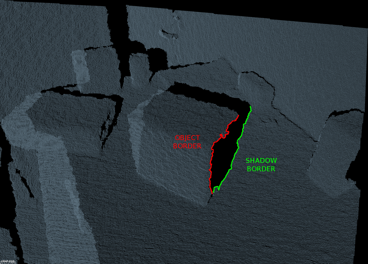
(左)境界の種類
(右)クラウドにおけるオブジェクト境界と影境界の例
このアルゴリズムは基本的に点の深度をその近傍の値と比較し、大きな差が見つかった場合、それが境界に起因することがわかる。 センサに近いポイントはオブジェクト境界としてマークされ、他のポイントは影境界としてマークされる。
PCLは、距離画像の境界線を抽出するクラスを提供している。
#include <pcl/io/pcd_io.h>
#include <pcl/range_image/range_image_planar.h>
#include <pcl/features/range_image_border_extractor.h>
#include <pcl/visualization/range_image_visualizer.h>

int
main(int argc, char** argv)
{
	// Object for storing the point cloud.  ポイントクラウドの記憶用のオブジェクト
	pcl::PointCloud<pcl::PointXYZ>::Ptr cloud(new pcl::PointCloud<pcl::PointXYZ>);
	// Object for storing the borders.  境界線の記憶用のオブジェクト
	pcl::PointCloud<pcl::BorderDescription>::Ptr borders(new pcl::PointCloud<pcl::BorderDescription>);

	// Read a PCD file from disk.   ハードディスクからPCDファイルを読み込む
	if (pcl::io::loadPCDFile<pcl::PointXYZ>(argv[1], *cloud) != 0)
	{
		return -1;
	}

	// Convert the cloud to range image.  クラウドを距離画像に変換
	int imageSizeX = 640, imageSizeY = 480;
	float centerX = (640.0f / 2.0f), centerY = (480.0f / 2.0f);
	float focalLengthX = 525.0f, focalLengthY = focalLengthX;
	Eigen::Affine3f sensorPose = Eigen::Affine3f(Eigen::Translation3f(cloud->sensor_origin_[0],
								 cloud->sensor_origin_[1],
								 cloud->sensor_origin_[2])) *
								 Eigen::Affine3f(cloud->sensor_orientation_);
	float noiseLevel = 0.0f, minimumRange = 0.0f;
	pcl::RangeImagePlanar rangeImage;
	rangeImage.createFromPointCloudWithFixedSize(*cloud, imageSizeX, imageSizeY,
			centerX, centerY, focalLengthX, focalLengthX,
			sensorPose, pcl::RangeImage::CAMERA_FRAME,
			noiseLevel, minimumRange);

	// Border extractor object.  境界抽出オブジェクト
	pcl::RangeImageBorderExtractor borderExtractor(&rangeImage);

	borderExtractor.compute(*borders);

	// Visualize the borders.  境界線の視覚化
	pcl::visualization::RangeImageVisualizer* viewer = NULL;
	viewer = pcl::visualization::RangeImageVisualizer::getRangeImageBordersWidget(rangeImage,
			 -std::numeric_limits<float>::infinity(),
			 std::numeric_limits<float>::infinity(),
			 false, *borders, "Borders");

	while (!viewer->wasStopped())
	{
		viewer->spinOnce();
		// Sleep 100ms to go easy on the CPU.  CPUでは100ms待つとよい
		pcl_sleep(0.1);
	}
}
 距離画像で見つかった境界
検出器の "getParameters()"関数を使用して、その設定値をもたせたpcl::RangeImageBorderExtractor::Parameters構造体を取得できる。
- 入力: 距離画像
- 出力: 境界
- Tutorial: How to extract borders from range images
- Publication:
- Bastian Steder et al. (2011) Point Feature Extraction on 3D Range Scans Taking into Account Object Boundaries
- API: pcl::RangeImageBorderExtractor
- Download
キーポイントの検索¶
Stederら(2011)の論文から引用:
「注目点の抽出手順について以下の要求を行っている:
1. 境界線や表面構造に関する情報を考慮していること
2. オブジェクトが別の視点から観測されたとしても、確実に検出できる位置を選択していること
3. 注目点は、法線推定や一般的に記述子の計算が安定した位置にあること
」
抽出手順は以下の通り:距離画像の各点に対し、その近傍で表面がどのくらい変化するかを表すスコアを計算する(サポートサイズ$\sigma$、つまり隣接する点を見つけるために使用される球の直径で近傍点を調整する)。また、この変化の支配的な方向も計算する。次に、この方向が近傍の点の方向と比較し、注目点の安定性を求める(これらの方向が非常に異なる場合、注目点は安定点ではなく、表面が大きく変化することを意味する)。オブジェクトのコーナー(エッジではないこと)の近くにあるポイントは良いキーポイントになるが、十分に安定した点である。
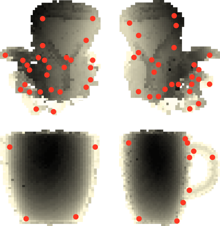
NARFキーポイント

上はサポートサイズ20cmの注目領域、下は1mの注目領域
PCLにはNARFキーポイントはこのようにして検出できる:
#include <pcl/io/pcd_io.h>
#include <pcl/range_image/range_image_planar.h>
#include <pcl/features/range_image_border_extractor.h>
#include <pcl/keypoints/narf_keypoint.h>
#include <pcl/visualization/range_image_visualizer.h>

int
main(int argc, char** argv)
{
	// Object for storing the point cloud. ポイントクラウドの記憶用のオブジェクト
	pcl::PointCloud<pcl::PointXYZ>::Ptr cloud(new pcl::PointCloud<pcl::PointXYZ>);
	// Object for storing the keypoints' indices. キーポイントのインデックス記憶用のオブジェクト
	pcl::PointCloud<int>::Ptr keypoints(new pcl::PointCloud<int>);

	// Read a PCD file from disk.  PCDファイルをハードディスクから読み込む
	if (pcl::io::loadPCDFile<pcl::PointXYZ>(argv[1], *cloud) != 0)
	{
		return -1;
	}

	// Convert the cloud to range image.  クラウドを距離画像に変換
	int imageSizeX = 640, imageSizeY = 480;
	float centerX = (640.0f / 2.0f), centerY = (480.0f / 2.0f);
	float focalLengthX = 525.0f, focalLengthY = focalLengthX;
	Eigen::Affine3f sensorPose = Eigen::Affine3f(Eigen::Translation3f(cloud->sensor_origin_[0],
								 cloud->sensor_origin_[1],
								 cloud->sensor_origin_[2])) *
								 Eigen::Affine3f(cloud->sensor_orientation_);
	float noiseLevel = 0.0f, minimumRange = 0.0f;
	pcl::RangeImagePlanar rangeImage;
	rangeImage.createFromPointCloudWithFixedSize(*cloud, imageSizeX, imageSizeY,
			centerX, centerY, focalLengthX, focalLengthX,
			sensorPose, pcl::RangeImage::CAMERA_FRAME,
			noiseLevel, minimumRange);

	pcl::RangeImageBorderExtractor borderExtractor;
	// Keypoint detection object.   キーポイント検出オブジェクト
	pcl::NarfKeypoint detector(&borderExtractor);
	detector.setRangeImage(&rangeImage);
	// The support size influences how big the surface of interest will be,
	// when finding keypoints from the border information.
    // サポートサイズは、境界情報からキーポイント検出の際、注目領域のサイズに影響する
	detector.getParameters().support_size = 0.2f;

	detector.compute(*keypoints);

	// Visualize the keypoints.  キーポイントの視覚化
	pcl::visualization::RangeImageVisualizer viewer("NARF keypoints");
	viewer.showRangeImage(rangeImage);
	for (size_t i = 0; i < keypoints->points.size(); ++i)
	{
		viewer.markPoint(keypoints->points[i] % rangeImage.width,
						 keypoints->points[i] / rangeImage.width,
						 // Set the color of the pixel to red (the background
						 // circle is already that color). All other parameters
						 // are left untouched, check the API for more options.
						 pcl::visualization::Vector3ub(1.0f, 0.0f, 0.0f));
	}

	while (!viewer.wasStopped())
	{
		viewer.spinOnce();
		// Sleep 100ms to go easy on the CPU.  CPUでは100ms待つと良い
		pcl_sleep(0.1);
	}
}

距離画像で見つかったNSRFキーポイント
- 入力: 距離画像、境界抽出器、サポートサイズ
- 出力: NARFキーポイント
- Publicaiton:
- Bastian Steder et al. (2011) Point Feature Extraction on 3D Range Scans Taking into Account Object Boundaries
- API: pcl::NarfKeypoint
- Download
記述子の計算¶
ポイントクラウドから距離画像を作成し、良好なキーポイントを見つけるために境界線を抽出した。 今度はキーポイントのNARF記述子を計算しよう。
NARF記述子は、ポイント周囲の表面変化についての情報をコード化する。 まず、この注目点の周辺に局所的なパッチを作成する。このパッチは注目点を中心とし法線に合わせた小さな範囲の画像のようなものである。 次に、n個のビームを有する星形パターンを注目点を中心として、このパッチ上に重ねる。 ビームごとに、その下の表面がどれだけ変化するかを反映する値を計算する。 変化が大きいほど、中心点に近いほど最終的な値は大きな値になる。 最終的な記述子は、n個の結果の値によって構成される。
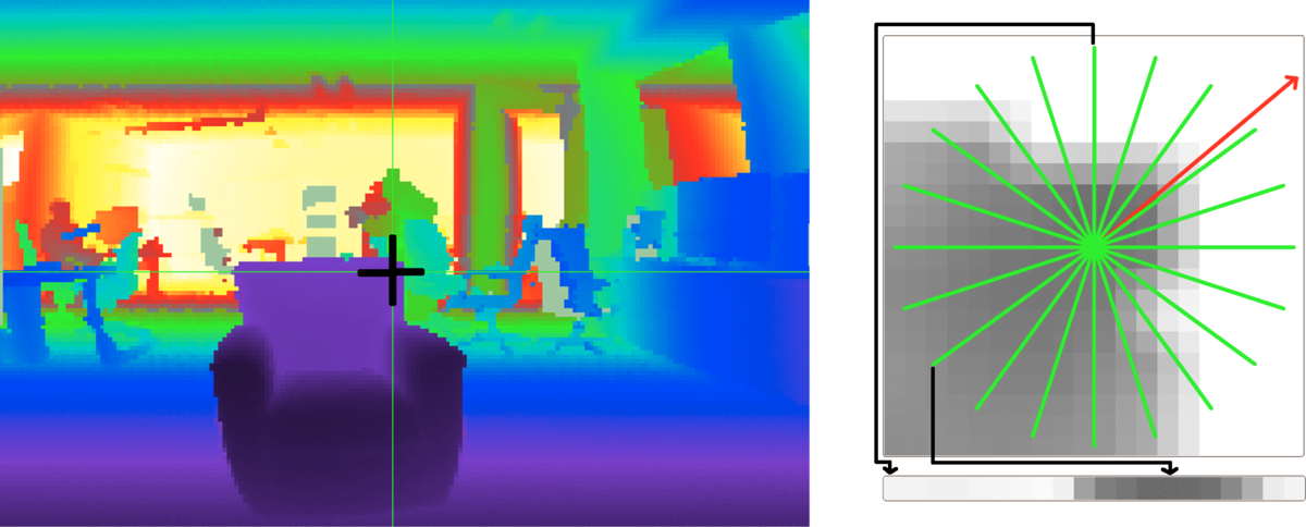 キーポイントに対するNARF記述子の計算
現在、この記述子は法線周りの回転に対して不変ではない。回転不変性を実現するために、360度全体をヒストグラムにビン詰めする。 各ビンの値は、角度に従って記述子の値から計算される。 次に、最も大きな値を持つビンを支配的な向きとみなし、それに従って記述子を変換する。
#include <pcl/io/pcd_io.h>
#include <pcl/range_image/range_image_planar.h>
#include <pcl/features/range_image_border_extractor.h>
#include <pcl/keypoints/narf_keypoint.h>
#include <pcl/features/narf_descriptor.h>

int
main(int argc, char** argv)
{
	// Object for storing the point cloud.   ポイントクラウド記憶用のオブジェクト
	pcl::PointCloud<pcl::PointXYZ>::Ptr cloud(new pcl::PointCloud<pcl::PointXYZ>);
	// Object for storing the keypoints' indices.  キーポイントのインデックスの記憶用のオブジェクト
	pcl::PointCloud<int>::Ptr keypoints(new pcl::PointCloud<int>);
	// Object for storing the NARF descriptors.  NARF記述子の記憶用のオブジェクト
	pcl::PointCloud<pcl::Narf36>::Ptr descriptors(new pcl::PointCloud<pcl::Narf36>);

	// Read a PCD file from disk.   ハードディスクからPCDファイルをファイルを読み込む
	if (pcl::io::loadPCDFile<pcl::PointXYZ>(argv[1], *cloud) != 0)
	{
		return -1;
	}

	// Convert the cloud to range image.  クラウドを距離画像に変換する
	int imageSizeX = 640, imageSizeY = 480;
	float centerX = (640.0f / 2.0f), centerY = (480.0f / 2.0f);
	float focalLengthX = 525.0f, focalLengthY = focalLengthX;
	Eigen::Affine3f sensorPose = Eigen::Affine3f(Eigen::Translation3f(cloud->sensor_origin_[0],
								 cloud->sensor_origin_[1],
								 cloud->sensor_origin_[2])) *
								 Eigen::Affine3f(cloud->sensor_orientation_);
	float noiseLevel = 0.0f, minimumRange = 0.0f;
	pcl::RangeImagePlanar rangeImage;
	rangeImage.createFromPointCloudWithFixedSize(*cloud, imageSizeX, imageSizeY,
			centerX, centerY, focalLengthX, focalLengthX,
			sensorPose, pcl::RangeImage::CAMERA_FRAME,
			noiseLevel, minimumRange);

	// Extract the keypoints.  キーポイントを抽出する
	pcl::RangeImageBorderExtractor borderExtractor;
	pcl::NarfKeypoint detector(&borderExtractor);
	detector.setRangeImage(&rangeImage);
	detector.getParameters().support_size = 0.2f;
	detector.compute(*keypoints);

	// The NARF estimator needs the indices in a vector, not a cloud.
    // NARF推定にはクラウドではなくベクトルの形でのインデックスが必要
	std::vector<int> keypoints2;
	keypoints2.resize(keypoints->points.size());
	for (unsigned int i = 0; i < keypoints->size(); ++i)
		keypoints2[i] = keypoints->points[i];
	// NARF estimation object.  NARF推定オブジェクト
	pcl::NarfDescriptor narf(&rangeImage, &keypoints2);
	// Support size: choose the same value you used for keypoint extraction.
    // サポートサイズ: キーポイント抽出のために使うのと同じ値を選ぶ
	narf.getParameters().support_size = 0.2f;
	// If true, the rotation invariant version of NARF will be used. The histogram
	// will be shifted according to the dominant orientation to provide robustness to
	// rotations around the normal.
    // true ならば、NARFの回転不変バージョンが使われる。法線周りの回転に対する頑健性を与えるため
    // 支配方向によってヒストグラムを変換する
	narf.getParameters().rotation_invariant = true;

	narf.compute(*descriptors);
}
- 入力: 距離画像、キーポイント、サポートサイズ
- 出力: NARF記述子
- Tutorial: How to extract NARF Features from a range image
- Publication:
- Bastian Steder et al. (2011) Point Feature Extraction on 3D Range Scans Taking into Account Object Boundaries
- API: pcl::NarfDescriptor
- Download
RoPS¶
Rotational Projection Statistics(RoPS, 回転投影統計)特徴量は他の記述子とは少し異なり、三角形メッシュで動作するため、クラウドからメッシュを生成するために前に述べた三角形分割処理が必要である。これ以外は他の記述子とほぼ似ている。
RoPSのキーポイントを計算するために、局所表面をサポート半径に沿って切り取る。そしてその内側にあるポイントと三角領域だけを考える。次に、局所参照座標系(LRF)を求め、それにより記述子に回転不変性を与える。対象ポイントを原点とし、軸をLRFに合わせた座標系を作成する。そして、すべての軸に対し、次のような処理を行う。
まず、局所表面を対象とする軸を中心に回転させる。その回転角度は、回転数を設定するパラメータの1つによって決まる。次に、局所表面のすべての点をXY平面、XZ平面、YZ平面に投影する。それぞれの投影点に対し、投影点の分布に関する統計情報を計算し、それを連結して最終的な記述子を形成する。
#include <pcl/io/pcd_io.h>
#include <pcl/point_types_conversion.h>
#include <pcl/features/normal_3d.h>
#include <pcl/surface/gp3.h>
#include <pcl/features/rops_estimation.h>

// A handy typedef.  便利な構造体宣言
typedef pcl::Histogram<135> ROPS135;

int
main(int argc, char** argv)
{
	// Object for storing the point cloud.     ポイントクラウドの格納用オブジェクト
	pcl::PointCloud<pcl::PointXYZ>::Ptr cloud(new pcl::PointCloud<pcl::PointXYZ>);
	// Object for storing the normals.      法線の推定
	pcl::PointCloud<pcl::Normal>::Ptr normals(new pcl::PointCloud<pcl::Normal>);
	// Object for storing both the points and the normals.  ポイントと法線両方の格納用オブジェクト
	pcl::PointCloud<pcl::PointNormal>::Ptr cloudNormals(new pcl::PointCloud<pcl::PointNormal>);
	// Object for storing the ROPS descriptor for each point. 各ポイントに対するROPS記述子の格納用オブジェクト
	pcl::PointCloud<ROPS135>::Ptr descriptors(new pcl::PointCloud<ROPS135>());

	// Read a PCD file from disk.   ハードディスクからPCDファイルを読み込む
	if (pcl::io::loadPCDFile<pcl::PointXYZ>(argv[1], *cloud) != 0)
	{
		return -1;
	}

	// Estimate the normals.     法線の推定
	pcl::NormalEstimation<pcl::PointXYZ, pcl::Normal> normalEstimation;
	normalEstimation.setInputCloud(cloud);
	normalEstimation.setRadiusSearch(0.03);
	pcl::search::KdTree<pcl::PointXYZ>::Ptr kdtree(new pcl::search::KdTree<pcl::PointXYZ>);
	normalEstimation.setSearchMethod(kdtree);
	normalEstimation.compute(*normals);

	// Perform triangulation.     三角形分割を行う
	pcl::concatenateFields(*cloud, *normals, *cloudNormals);
	pcl::search::KdTree<pcl::PointNormal>::Ptr kdtree2(new pcl::search::KdTree<pcl::PointNormal>);
	kdtree2->setInputCloud(cloudNormals);
	pcl::GreedyProjectionTriangulation<pcl::PointNormal> triangulation;
	pcl::PolygonMesh triangles;
	triangulation.setSearchRadius(0.025);
	triangulation.setMu(2.5);
	triangulation.setMaximumNearestNeighbors(100);
	triangulation.setMaximumSurfaceAngle(M_PI / 4); // 45 degrees. 45度をラディアンで
	triangulation.setNormalConsistency(false);
	triangulation.setMinimumAngle(M_PI / 18); // 10 degrees.   10度をラディアンで
	triangulation.setMaximumAngle(2 * M_PI / 3); // 120 degrees. 120度をラディアンで
	triangulation.setInputCloud(cloudNormals);
	triangulation.setSearchMethod(kdtree2);
	triangulation.reconstruct(triangles);

	// Note: you should only compute descriptors for chosen keypoints. It has
	// been omitted here for simplicity.
    // 注意: 普通はここでダウンサンプリングを行う。このコードでは省略しているが、時間がかかることに注意

	// RoPs estimation object.  RoPs推定オブジェクト
	pcl::ROPSEstimation<pcl::PointXYZ, ROPS135> rops;
	rops.setInputCloud(cloud);
	rops.setSearchMethod(kdtree);
	rops.setRadiusSearch(0.03);
	rops.setTriangles(triangles.polygons);
	// Number of partition bins that is used for distribution matrix calculation.
    // 分散行列計算に用いられる分割ビンの個数
	rops.setNumberOfPartitionBins(5);
	// The greater the number of rotations is, the bigger the resulting descriptor.
	// Make sure to change the histogram size accordingly.
    // 回転数が多いほど結果として得られる記述子が大きくなる。それに合わせてヒストグラムのサイズを変更すること
	rops.setNumberOfRotations(3);
	// Support radius that is used to crop the local surface of the point.
    // サポート半径はポイントの局所表面を切り取るのに用いられる
	rops.setSupportRadius(0.025);

	rops.compute(*descriptors);
}
- 入力: ポイント、三角形分割、探索手法、サポート半径、回転数、分割ビンの個数
- 出力: RoPS 記述子
- Publication:
- Yulan Guo et al. (2013) Rotational Projection Statistics for 3D Local Surface Description and Object Recognition
- API: pcl::ROPSEstimation
- Download
大局記述子¶
大局記述子は物体の幾何形状ををコード化するものである。つまり、個々の点について計算されるものではなく、物体を表すクラスタ全体に対して計算されるものである。 このため、可能な候補を得るために、前処理ステップ(セグメンテーション)が必要である。
大局記述子は、物体認識と分類、幾何学的解析(物体のタイプ、形状...)、姿勢推定に使用される。
局所記述子の多くも大局記述子として使用できることも知っておこう。 これは、(PFHのように)近傍点検索のために探索半径を使用する記述子が該当する。そのトリックは、オブジェクトクラスタ内のただ一点について局所記述子を求め、任意の2点間の最大距離に探索半径を設定するのである(これにより、クラスタ内のすべての点が隣接点とみなされる)。
VFH¶
Viewpoint Feature Histogram (VFH, 視点特徴量ヒストグラム)は、FPFHに基づく記述子である。FPFHは物体の姿勢に対して不変なので、提案者は視点についての情報を含める拡張を行った。また、FPFHはすべてのポイントではなくクラスタ全体に対して1回だけ推定されるため効率的である。
VFHは、視点方向成分と拡張FPFH成分という2つの部分で構成されている。視点方向成分を計算するために、オブジェクトの重心を求める。重心とはすべての点のX、Y、Z座標の平均を座標とする点である。次いで、視点(センサの位置)とこの重心との間のベクトルが計算され、正規化される。最後に、クラスタ内のすべての点について、このベクトルと法線との間の角度が計算され、その結果がヒストグラムで表される。ポイントと重心とのベクトルは角度計算において各ポイントに対して正規化するため、記述子はスケール不変になる。
拡張FPFH成分はFPFHと同様に計算される(3つの角度特徴量、$\alpha, \phi, \theta$のヒストグラムが得られる)。ただしいくつか違いがある。前の計算で得られた視点方向ベクトルを法線とし(明らかに対象ポイントは法線を持たない)、すべてのクラスタのポイントを近傍点としているのである。


(左) VFHの視点方向成分
(右) 拡張FPFH成分
得られた4つのヒストグラム(視点成分が1個、拡張FPFH成分は3個)を連結して最終的なVFH記述子を構築する。 デフォルトでは、ビンはクラスタ内の合計ポイント数を使用して正規化する。 これにより、VFH記述子はスケール不変となる。
 VFHヒストグラム
PCLの実装では、クラスターのポイントから重心までの距離(SDC、形状分布成分)のヒストグラムを計算し5番目のヒストグラムとして追加しているので、出力記述子のサイズは263から308に増えている。SDCは次節で述べるCVFH記述子から得られ、結果はより頑健になる。
前もってクラスター化したオブジェクトのVFHは、次のように計算できる:
#include <pcl/io/pcd_io.h>
#include <pcl/features/normal_3d.h>
#include <pcl/features/vfh.h>

int
main(int argc, char** argv)
{
	// Cloud for storing the object.  クラウド格納用のオブジェクト
	pcl::PointCloud<pcl::PointXYZ>::Ptr object(new pcl::PointCloud<pcl::PointXYZ>);
	// Object for storing the normals.  法線を格納用のオブジェクト
	pcl::PointCloud<pcl::Normal>::Ptr normals(new pcl::PointCloud<pcl::Normal>);
	// Object for storing the VFH descriptor. VFH記述子格納用のオブジェクト
	pcl::PointCloud<pcl::VFHSignature308>::Ptr descriptor(new pcl::PointCloud<pcl::VFHSignature308>);

	// Note: you should have performed preprocessing to cluster out the object
	// from the cloud, and save it to this individual file.
    // 注意: クラウドからオブジェクトを切り出すという前処理を実行し、これを個々のファイルに格納すべき

	// Read a PCD file from disk. ハードディスクからPCDファイルを読み込む
	if (pcl::io::loadPCDFile<pcl::PointXYZ>(argv[1], *object) != 0)
	{
		return -1;
	}

	// Estimate the normals. 法線の推定
	pcl::NormalEstimation<pcl::PointXYZ, pcl::Normal> normalEstimation;
	normalEstimation.setInputCloud(object);
	normalEstimation.setRadiusSearch(0.03);
	pcl::search::KdTree<pcl::PointXYZ>::Ptr kdtree(new pcl::search::KdTree<pcl::PointXYZ>);
	normalEstimation.setSearchMethod(kdtree);
	normalEstimation.compute(*normals);

	// VFH estimation object.  VFH推定のオブジェクト
	pcl::VFHEstimation<pcl::PointXYZ, pcl::Normal, pcl::VFHSignature308> vfh;
	vfh.setInputCloud(object);
	vfh.setInputNormals(normals);
	vfh.setSearchMethod(kdtree);
	// Optionally, we can normalize the bins of the resulting histogram,
	// using the total number of points.
    // 任意で、結果として得られたヒストグラムのビンをポイントの総数で正規化できる
	vfh.setNormalizeBins(true);
	// Also, we can normalize the SDC with the maximum size found between
	// the centroid and any of the cluster's points.
    // また重心とクラスタのポイントの最大サイズでSDCを正規化することも可能
	vfh.setNormalizeDistance(false);

	vfh.compute(*descriptor);
}
クラスタ全体に対し1つのVFH記述子しか計算されないため、結果を格納するクラウドオブジェクトのサイズは1になる。
- 入力: ポイント(クラスタ)、法線、探索手法、(正規化ビン), (正規化SDC)(cluster)
- 出力: VFH 記述子
- Tutorial: Estimating VFH signatures for a set of points
- Publication:
- Radu Bogdan Rusu et al.(2010)Fast 3D Recognition and Pose Using the Viewpoint Feature Histogram
- API: pcl::VFHEstimation
- Download
CVFH¶
元々のVFH記述子は、オクルージョンやセンサ誤差、測定誤りに対して頑健ではない。 オブジェクトクラスタにポイントが多く失われている場合、計算結果の重心は本当の値とは異なり、最終的な記述子を変化させ、その結果見つけられるべき一致が得られなくなる。そのため、 Clustered Viewpoint Feature Histogram(CVFH、クラスタ化視点特徴量ヒストグラム)が提案された。
アイデアは非常に単純である:クラスタ全体に対し一個のVFHヒストグラムを計算する代わりに、最初に、領域成長セグメンテーションを使用して安定した滑らかな領域にオブジェクトを分割し、個々の領域に属す点の法線の距離と差に制約を課す。次に、それぞれの領域に対しVFHを求める。 これにより、その領域の一つでも完全に見えるのであれば、シーン内でオブジェクトを見つけることができる。


(左)ポイントクラウドにおける典型的なオクルージョン問題
(右)CVFH用に計算されたオブジェクト領域
さらに、形状分布コンポーネント(SDC)も計算され、含められる。 SDCは、距離を測定し、領域の重心周りの点の分布に関する情報を符号化している。 SDCを使用すると、類似の特性(サイズと正規分布)を持つオブジェクト(例えば2つの平面)を区別することができる。
著者は、VFHで実行されるヒストグラムの正規化処理の破棄を提案している。 これは、記述子がスケールに依存させる効果があるため、特定のサイズのオブジェクトは、それ自身より大きいか小さいコピーと一致しない。 また、CVFHをオクルージョンに対してより頑健にする。
CVFHは、ほとんどの大局記述子と同様に、カメラのロール角に対して不変である。そうなる理由は、カメラ軸に関する回転は、記述子を計算する観測可能な幾何形状を変更せず、姿勢推定を5 DoF(自由度)に制限するためである。 これを克服するために、カメラロールヒストグラム(CRH)の使用が提案されている。
#include <pcl/io/pcd_io.h>
#include <pcl/features/normal_3d.h>
#include <pcl/features/cvfh.h>

int
main(int argc, char** argv)
{
	// Cloud for storing the object.  クラウド格納用のオブジェクト
	pcl::PointCloud<pcl::PointXYZ>::Ptr object(new pcl::PointCloud<pcl::PointXYZ>);
	// Object for storing the normals.  法線格納用のオブジェクト
	pcl::PointCloud<pcl::Normal>::Ptr normals(new pcl::PointCloud<pcl::Normal>);
	// Object for storing the CVFH descriptors.  CVFH記述子格納用のオブジェクト
	pcl::PointCloud<pcl::VFHSignature308>::Ptr descriptors(new pcl::PointCloud<pcl::VFHSignature308>);

	// Note: you should have performed preprocessing to cluster out the object
	// from the cloud, and save it to this individual file.
    // 注意: クラウドからオブジェクトを切り出すという前処理を実行し、これを個々のファイルに格納すべき

	// Read a PCD file from disk.  ハードディスクからPCDファイルを読み込む
	if (pcl::io::loadPCDFile<pcl::PointXYZ>(argv[1], *object) != 0)
	{
		return -1;
	}

	// Estimate the normals.  法線の推定
	pcl::NormalEstimation<pcl::PointXYZ, pcl::Normal> normalEstimation;
	normalEstimation.setInputCloud(object);
	normalEstimation.setRadiusSearch(0.03);
	pcl::search::KdTree<pcl::PointXYZ>::Ptr kdtree(new pcl::search::KdTree<pcl::PointXYZ>);
	normalEstimation.setSearchMethod(kdtree);
	normalEstimation.compute(*normals);

	// CVFH estimation object.  CVFH推定オブジェクト
	pcl::CVFHEstimation<pcl::PointXYZ, pcl::Normal, pcl::VFHSignature308> cvfh;
	cvfh.setInputCloud(object);
	cvfh.setInputNormals(normals);
	cvfh.setSearchMethod(kdtree);
	// Set the maximum allowable deviation of the normals,
	// for the region segmentation step.
    // 領域セグメンテーションのため、法線の許容可能な最大偏差を設定
	cvfh.setEPSAngleThreshold(5.0 / 180.0 * M_PI); // 5 degrees.
	// Set the curvature threshold (maximum disparity between curvatures),
	// for the region segmentation step.
    // 領域セグメンテーションのため、曲率の閾値(曲率の最大差)の設定
	cvfh.setCurvatureThreshold(1.0);
	// Set to true to normalize the bins of the resulting histogram,
	// using the total number of points. Note: enabling it will make CVFH
	// invariant to scale just like VFH, but the authors encourage the opposite.
    // trueであれば、ポイントの総数を用いて結果として得られるヒストグラムのビンを正規化する
    // 注意: これを可能にすると、CVFHはVFHのようにスケール不変になるが、著者はそうしないよう勧めている
	cvfh.setNormalizeBins(false);

	cvfh.compute(*descriptors);
}
"setClusterTolerance()"(同じクラスタ内のポイント間の最大ユークリッド距離を設定する)と "setMinPoints()"を使用して、セグメンテーション処理をさらにカスタマイズできる。 出力のサイズは、オブジェクトが分割された領域の数に等しくなる。また、関数 "getCentroidClusters()"と "getCentroidNormalClusters()"により、いろいろなCVFH記述子の計算に用いる重心の情報が得られる。
- 入力: ポイント(クラスタ), 法線、探索手法、角度の閾値、曲率の閾値、(法線ビン)、(クラスタ許容度)、(最小ポイント)
- 出力: CVFH記述子
- Publication:
- Aitor Aldoma et al. (2011) CAD-Model Recognition and 6DOF Pose Estimation Using 3D Cues (requires IEEE Xplore subscription)
- API: pcl::CVFHEstimation
- Download
OUR-CVFH¶
Oriented Unique Repeatable CVFH(OUR-CVFH、指向的一意的反復可能なCVFH) は前節で述べたCVFH記述子を拡張し、一意的な参照座標系の計算を加えて頑健性を高めたものである。
OUR-CVFHはSemi-Global Unique Reference Frame (SGURF, 半大局的一意的参照座標系)によるものである。SGURFは領域ごとに計算される反復可能な座標系である。これによりカメラのロール角への不変性が除去されるだけでなく、6DoF(6自由度)のカメラ姿勢が追加処理なしで直接取り出せ、空間的な記述力をも向上させる。
この計算の最初の部分はCVFHに似ているが、セグメンテーション後、それぞれの領域のポイントは、法線と領域の平均法線の差により再度フィルタリングされる。これにより、より良い形状の領域が得られ、参照座標系(RF)の推定が改善される。
その後、SGURFは領域ごとに計算される。点の分布に基づいて軸の正負の符号を決定するため、曖昧さ除去を行う。これが十分ではなく符号の決定に曖昧さが残った場合は、複数のRFを作成する必要がある。最後に、OUR-CVFH記述子が計算される。本来の形状分布コンポーネント(SDC)は破棄され、表面形状はRFに従って記述されるようになる。
 ある領域のSGURF座標系と結果として得られるヒストグラム
#include <pcl/io/pcd_io.h>
#include <pcl/features/normal_3d.h>
#include <pcl/features/our_cvfh.h>

int
main(int argc, char** argv)
{
	// Cloud for storing the object. クラウド記憶用のオブジェクト
	pcl::PointCloud<pcl::PointXYZ>::Ptr object(new pcl::PointCloud<pcl::PointXYZ>);
	// Object for storing the normals. 法線記憶用のオブジェクト
	pcl::PointCloud<pcl::Normal>::Ptr normals(new pcl::PointCloud<pcl::Normal>);
	// Object for storing the OUR-CVFH descriptors. OUR-CVFH記述子のためのオブジェクト
	pcl::PointCloud<pcl::VFHSignature308>::Ptr descriptors(new pcl::PointCloud<pcl::VFHSignature308>);

	// Note: you should have performed preprocessing to cluster out the object
	// from the cloud, and save it to this individual file.
    // 注意: クラウドからオブジェクトを切り出すという前処理を実行し、これを個々のファイルに格納すべき
	// Read a PCD file from disk.  ハードディスクからPCDファイルを読み込む
	if (pcl::io::loadPCDFile<pcl::PointXYZ>(argv[1], *object) != 0)
	{
		return -1;
	}

	// Estimate the normals. 法線の推定
	pcl::NormalEstimation<pcl::PointXYZ, pcl::Normal> normalEstimation;
	normalEstimation.setInputCloud(object);
	normalEstimation.setRadiusSearch(0.03);
	pcl::search::KdTree<pcl::PointXYZ>::Ptr kdtree(new pcl::search::KdTree<pcl::PointXYZ>);
	normalEstimation.setSearchMethod(kdtree);
	normalEstimation.compute(*normals);

	// OUR-CVFH estimation object.  OUR=CVFH推定オブジェクト
	pcl::OURCVFHEstimation<pcl::PointXYZ, pcl::Normal, pcl::VFHSignature308> ourcvfh;
	ourcvfh.setInputCloud(object);
	ourcvfh.setInputNormals(normals);
	ourcvfh.setSearchMethod(kdtree);
	ourcvfh.setEPSAngleThreshold(5.0 / 180.0 * M_PI); // 5 degrees.
	ourcvfh.setCurvatureThreshold(1.0);
	ourcvfh.setNormalizeBins(false);
	// Set the minimum axis ratio between the SGURF axes. At the disambiguation phase,
	// this will decide if additional Reference Frames need to be created, if ambiguous.
	ourcvfh.setAxisRatio(0.8);

	ourcvfh.compute(*descriptors);
}
getTransforms()関数を使用して、対応するSGURFにクラウドを合わせる変換を取得できる。
- 入力: ポイント(クラスタ), 法線、探索手法、角度の閾値、曲率の閾値、(法線ビン)、(クラスタ許容度)、(最小ポイント), (軸割合)
- 出力: OUR-CVFH 記述子
- Publication:
- API: pcl::OURCVFHEstimation
- Download
ESF¶
ESF(Ensemble of Shape Functions、形状関数のアンサンブル)は、クラウドのポイントの特定の特性(距離、角度、面積)を記述する3つの異なる形状関数の組み合わせである。この記述子は、法線情報を必要としないユニークな記述子である。実際には、ノイズや不完全な表面に強いため、前処理を必要としない。
このアルゴリズムは、実表面の近似としてボクセル・グリッドを使用する。クラウド内のすべてのポイントを反復処理する。反復ごとにランダムに3つのポイントを選び、これらのポイントに対し形状関数を計算する。
- D2:この関数はポイント対間の距離を計算する(全部で3個)。次に、各ペアについて、両方の点を結ぶ線が完全に面の内側にあるか、完全に外側にあるか(自由空間と交差する)か、またはどちらでもないかを調べる。これによって、距離値を3つのヒストグラム(IN、OUT、MIXED)のいずれかにビニングする。
- D2比:ポイント対間の線の表面内部の部分と外部の部分との比のヒストグラム。この値は、線が完全に外側にある場合は0、完全に内側の場合は1、混合の(どちらでもない)場合は比の値である。
- D3:3点で作られる三角形の面積の平方根を計算する。 D2と同様に結果はIN、OUT、MIXEDに分類され、それぞれ独自のヒストグラムがある。
- A3:この関数はポイントによって作られる角度を計算し、その角と(三角形において)向かい合う辺の線分がどうか(またもやIN、OUT、MIXED)によりビニングする。
 ESF記述子
反復処理が終了すると、10個のヒストグラムができあがる(D2、D3、A3においてIN、OUT、MIXEDの3個ずつ、比率で1個)。 それぞれに64個のビンがあるので、最終的なESF記述子のサイズは640である。
#include <pcl/io/pcd_io.h>
#include <pcl/features/esf.h>

int
main(int argc, char** argv)
{
	// Cloud for storing the object.    クラウド記憶用のオブジェクト
	pcl::PointCloud<pcl::PointXYZ>::Ptr object(new pcl::PointCloud<pcl::PointXYZ>);
	// Object for storing the ESF descriptor.   ESP記述子のためのオブジェクト
	pcl::PointCloud<pcl::ESFSignature640>::Ptr descriptor(new pcl::PointCloud<pcl::ESFSignature640>);

	// Note: you should have performed preprocessing to cluster out the object
	// from the cloud, and save it to this individual file.
    // 注意: クラウドからオブジェクトを切り出すという前処理を実行し、これを個々のファイルに格納すべき

	// Read a PCD file from disk. ハードディスクからPCDファイルを読み込む
	if (pcl::io::loadPCDFile<pcl::PointXYZ>(argv[1], *object) != 0)
	{
		return -1;
	}

	// ESF estimation object.     ESF推定のオブジェクト
	pcl::ESFEstimation<pcl::PointXYZ, pcl::ESFSignature640> esf;
	esf.setInputCloud(object);

	esf.compute(*descriptor);
}
- 入力: ポイント(クラスタ)
- 出力: ESF 記述子
- Publication:
- Walter Wohlkinger & Markus Vincze (2011) Ensemble of shape functions for 3D object classification (requires IEEE Xplore subscription)
- API: pcl::ESFEstimation
- Download
GFPFH¶
GFPFHはGlobal Fast Point Feature Histogram(大局的高速ポイント特徴量ヒストグラム)の略であり、FPFH記述子の大局バージョンである。 GFPFHは環境内におけるロボットの移動支援のために設計されており、周囲のオブジェクトの情報を持っている。
記述子計算のための最初のステップは、表面の分類である。ロボットがシーンで検出すると予想されるオブジェクトのタイプに応じて、論理プリミティブ(クラス、つまりカテゴリ)のセットを作成しておく。 たとえば、コーヒーマグがあることが分かっている場合は、マグの取っ手とマグの外面と内面の合計3つのカテゴリを作成する。 次に、FPFH記述子を計算し、これを条件付きランダム・フィールド(CRF)アルゴリズムに入力する。 CRFは各サーフェスにカテゴリの1つを割り当てる。そのため、各ポイントが属すオブジェクト(またはオブジェクト領域)のタイプによって分類されるクラウドが最終的に得られる。
 FPFHとCRFによるオブジェクト分類
こで、GFPFH記述子は、分類ステップの結果を用いて計算することができる。 オブジェクトが何を構成しているかをエンコードするので、ロボットは簡単に認識できます。 最初に、オクツリーが作成され、ボクセルの葉のオブジェクトを分割します。 すべてのリーフに対して、クラスごとに1つの確率のセットが作成されます。 それぞれは、そのクラスに属するリーフの確率を格納し、そのクラスとしてラベル付けされたそのリーフ内のポイントの数および合計ポイント数に従って計算される。 次に、オクトリー内の葉のペアごとに、ラインがキャストされ、それらを接続します。 そのパス内のすべてのリーフが占有をチェックされ、その結果がヒストグラムに格納されます。 リーフが空(空き領域)の場合、値0が保存されます。 それ以外の場合は、リーフ確率が使用されます。
 ボクセルグリッドによるGFPFHの計算
次のコードは、ラベル情報を持つクラウドのGFPFHを計算する。オブジェクトの分類処理は、シーンの種類と使用用途に大きく依存する。
#include <pcl/io/pcd_io.h>
#include <pcl/features/gfpfh.h>

int
main(int argc, char** argv)
{
	// Cloud for storing the object.  クラウド記憶用のオブジェクト
	pcl::PointCloud<pcl::PointXYZL>::Ptr object(new pcl::PointCloud<pcl::PointXYZL>);
	// Object for storing the GFPFH descriptor.  GFPFH記述子記憶用のオブジェクト
	pcl::PointCloud<pcl::GFPFHSignature16>::Ptr descriptor(new pcl::PointCloud<pcl::GFPFHSignature16>);

	// Note: you should have performed preprocessing to cluster out the object
	// from the cloud, and save it to this individual file.
    // 注意: クラウドからオブジェクトを切り出すという前処理を実行し、これを個々のファイルに格納すべき
	// Read a PCD file from disk.   ハードディスクからPCDファイルを読み込む
	if (pcl::io::loadPCDFile<pcl::PointXYZL>(argv[1], *object) != 0)
	{
		return -1;
	}

	// Note: you should now perform classification on the cloud's points. See the
	// original paper for more details. For this example, we will now consider 4
	// different classes, and randomly label each point as one of them.
    // 注意: ここでクラウドのポイントに対しオブジェクト分類を実行すべきである
    // 詳細については原著論文を参照のこと。この例では4個のクラスを考え、
    // 各ポイントに対しランダムにクラスをラベル付している
	for (size_t i = 0; i < object->points.size(); ++i)
	{
		object->points[i].label = 1 + i % 4;
	}

	// ESF estimation object.  ESF推定オブジェクト
	pcl::GFPFHEstimation<pcl::PointXYZL, pcl::PointXYZL, pcl::GFPFHSignature16> gfpfh;
	gfpfh.setInputCloud(object);
	// Set the object that contains the labels for each point. Thanks to the
	// PointXYZL type, we can use the same object we store the cloud in.
    // それぞれのポイントに対するラベルを持つオブジェクトを設定。
    // PointXYZL型のおかげで、クラウドを記憶する同じオブジェクトをそのために使える
	gfpfh.setInputLabels(object);
	// Set the size of the octree leaves to 1cm (cubic). 八分木の葉のサイズを1cm(立方)に設定
	gfpfh.setOctreeLeafSize(0.01);
	// Set the number of classes the cloud has been labelled with (default is 16).
    // クラウドがラベル付されるクラスの個数を設定(デフォルトは16, この例では4)
	gfpfh.setNumberOfClasses(4);

	gfpfh.compute(*descriptor);
}
- 入力: ポイント(クラスタ)、ラベル、クラスの個数、葉のサイズ
- 出力: GFPFH 記述子
- Publication:
- Radu Bogdan Rusu et al. (2009) Detecting and Segmenting Objects for Mobile Manipulation
- API: pcl::GFPFHEstimation
- Download
GRSD¶
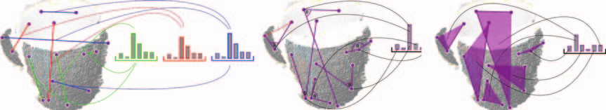
GRSDは、RSD(半径系表面記述子)の大局バージョンであり、GFPFHと同様に動作する。 RSDを使用して、ボクセル化および表面分類処理を事前に実行しておき、幾何学的カテゴリ(平面、円柱、エッジ、へり(周縁)、球)に基づきすべての表面パッチにラベルづけする。 次に、クラスタ全体をこのカテゴリの1つに分類し、これからGRSD記述子を求める。
 GRSDのためのオブジェクト分類とその結果得られるヒストグラム
#include <pcl/io/pcd_io.h>
#include <pcl/features/normal_3d.h>
#include <pcl/features/grsd.h>

int
main(int argc, char** argv)
{
	// Object for storing the point cloud.   ポイントクラウド記憶用のオブジェクト
	pcl::PointCloud<pcl::PointXYZ>::Ptr cloud(new pcl::PointCloud<pcl::PointXYZ>);
	// Object for storing the normals.   法線記憶用のオブジェクト
	pcl::PointCloud<pcl::Normal>::Ptr normals(new pcl::PointCloud<pcl::Normal>);
	// Object for storing the GRSD descriptors for each point.  各ポイントに対するGRSD記述子記憶用のオブジェクト
	pcl::PointCloud<pcl::GRSDSignature21>::Ptr descriptors(new pcl::PointCloud<pcl::GRSDSignature21>());

	// Read a PCD file from disk.  PCDファイルをハードディスクから読み込む
	if (pcl::io::loadPCDFile<pcl::PointXYZ>(argv[1], *cloud) != 0)
	{
		return -1;
	}

	// Note: you would usually perform downsampling now. It has been omitted here
	// for simplicity, but be aware that computation can take a long time.
    // 注意: 普通はここでダウンサンプリングを行う。このコードでは省略しているが、時間がかかることに注意
	// Estimate the normals.  法線の推定
	pcl::NormalEstimation<pcl::PointXYZ, pcl::Normal> normalEstimation;
	normalEstimation.setInputCloud(cloud);
	normalEstimation.setRadiusSearch(0.03);
	pcl::search::KdTree<pcl::PointXYZ>::Ptr kdtree(new pcl::search::KdTree<pcl::PointXYZ>);
	normalEstimation.setSearchMethod(kdtree);
	normalEstimation.compute(*normals);

	// GRSD estimation object.  GRSD推定オブジェクト
	pcl::GRSDEstimation<pcl::PointXYZ, pcl::Normal, pcl::GRSDSignature21> grsd;
	grsd.setInputCloud(cloud);
	grsd.setInputNormals(normals);
	grsd.setSearchMethod(kdtree);
	// Search radius, to look for neighbors. Note: the value given here has to be
	// larger than the radius used to estimate the normals.
    // 近傍点を探すための探索半径、注意: この値は法線推定のため半径よりも大きくなければならない
	grsd.setRadiusSearch(0.05);

	grsd.compute(*descriptors);
}
注:このコードはPCLバージョン1.8以上(現在のバージョン)でのみコンパイル可能。
- 入力: ポイント(クラスタ)、法線、探索手法、半径
- 出力: GRSD 記述子
- Publications:
- Zoltan-Csaba Marton et al. (2010) Hierarchical Object Geometric Categorization and Appearance Classification for Mobile Manipulation
- Zoltan-Csaba Marton et al. (2011) Combined 2D-3D Categorization and Classification for Multimodal Perception Systems
- Zoltan-Csaba Marton et al. (2011) Voxelized Shape and Color Histograms for RGB-D
- API: pcl::GRSDEstimation
- Download
保存と読み込み¶
他のクラウドタイプと同様に、記述子をファイルに保存できる。 しかしここで警告。 "PFHSignature125"のような独自のカスタムタイプを持つ記述子を使用している場合は問題ないが、そうでない場合("pcl::Histogram <>"を使用しなければならない場合)"POINT_TYPE_NOT_PROPERLY_REGISTERED"(ポイントの型が適正に登録されていない)というエラーが発生する。 PCLのIO(入出力)機能は、ファイルを保存したり読み込んだりするために、フィールドの数、タイプ、サイズを知る必要がある。 これを解決するには、使用する記述子に対するポイントタイプを正しく登録する必要がある。 たとえば、これは前に見たRoPS記述子の例ではうまくいく:
POINT_CLOUD_REGISTER_POINT_STRUCT(ROPS135,
                                  (float[135], histogram, histogram)
)
上のコードをコードに追加(それに応じて変更する)すると、記述子を保存したり読み込んだりできる。
#include <pcl/io/pcd_io.h>
#include <pcl/features/normal_3d.h>
#include <pcl/features/vfh.h>
#include<pcl/visualization/histogram_visualizer.h>

int
main(int argc, char** argv)
{
	// Clouds for storing everything.  すべてを記憶するためのクラウド
	pcl::PointCloud<pcl::PointXYZ>::Ptr object(new pcl::PointCloud<pcl::PointXYZ>);
	pcl::PointCloud<pcl::Normal>::Ptr normals(new pcl::PointCloud<pcl::Normal>);
	pcl::PointCloud<pcl::VFHSignature308>::Ptr descriptor(new pcl::PointCloud<pcl::VFHSignature308>);

	// Read a PCD file from disk.     PCDファイルをハードディスクから読み込む
	if (pcl::io::loadPCDFile<pcl::PointXYZ>(argv[1], *object) != 0)
	{
		return -1;
	}

	// Estimate the normals.   法線推定
	pcl::NormalEstimation<pcl::PointXYZ, pcl::Normal> normalEstimation;
	normalEstimation.setInputCloud(object);
	normalEstimation.setRadiusSearch(0.03);
	pcl::search::KdTree<pcl::PointXYZ>::Ptr kdtree(new pcl::search::KdTree<pcl::PointXYZ>);
	normalEstimation.setSearchMethod(kdtree);
	normalEstimation.compute(*normals);

	// Estimate VFH descriptor.   VFH記述子の推定
	pcl::VFHEstimation<pcl::PointXYZ, pcl::Normal, pcl::VFHSignature308> vfh;
	vfh.setInputCloud(object);
	vfh.setInputNormals(normals);
	vfh.setSearchMethod(kdtree);
	vfh.setNormalizeBins(true);
	vfh.setNormalizeDistance(false);
	vfh.compute(*descriptor);

	// Plotter object.   オブジェクトをプロット(描画)
	pcl::visualization::PCLHistogramVisualizer viewer;
	// We need to set the size of the descriptor beforehand.  予め記述子のサイズをセットする必要がある
	viewer.addFeatureHistogram(*descriptor, 308);

	viewer.spin();
}
 ヒストグラム視覚化で表示されたVFHヒストグラム
- 入力: 記述子、記述子のサイズ、(ウィンドゥのサイズ), (背景色), (Y軸の範囲)
- API: pcl::visualization::PCLHistogramVisualizer
- Download
PCLPlotter¶
このクラスには、 "PCLHistogramVisualizer"(廃止予定)のメソッドと、さらに多くの機能がある。 コードはほぼ同じである:
#include <pcl/io/pcd_io.h>
#include <pcl/features/normal_3d.h>
#include <pcl/features/vfh.h>
#include<pcl/visualization/pcl_plotter.h>

int
main(int argc, char** argv)
{
	// Clouds for storing everything.  すべてを記憶するためのクラウド
	pcl::PointCloud<pcl::PointXYZ>::Ptr object(new pcl::PointCloud<pcl::PointXYZ>);
	pcl::PointCloud<pcl::Normal>::Ptr normals(new pcl::PointCloud<pcl::Normal>);
	pcl::PointCloud<pcl::VFHSignature308>::Ptr descriptor(new pcl::PointCloud<pcl::VFHSignature308>);

	// Read a PCD file from disk.  PCDファイルをハードディスクから読み込む
	if (pcl::io::loadPCDFile<pcl::PointXYZ>(argv[1], *object) != 0)
	{
		return -1;
	}

	// Estimate the normals.   法線推定
	pcl::NormalEstimation<pcl::PointXYZ, pcl::Normal> normalEstimation;
	normalEstimation.setInputCloud(object);
	normalEstimation.setRadiusSearch(0.03);
	pcl::search::KdTree<pcl::PointXYZ>::Ptr kdtree(new pcl::search::KdTree<pcl::PointXYZ>);
	normalEstimation.setSearchMethod(kdtree);
	normalEstimation.compute(*normals);

	// Estimate VFH descriptor.  VFH記述子の推定
	pcl::VFHEstimation<pcl::PointXYZ, pcl::Normal, pcl::VFHSignature308> vfh;
	vfh.setInputCloud(object);
	vfh.setInputNormals(normals);
	vfh.setSearchMethod(kdtree);
	vfh.setNormalizeBins(true);
	vfh.setNormalizeDistance(false);
	vfh.compute(*descriptor);

	// Plotter object.  オブジェクトのプロット
	pcl::visualization::PCLPlotter plotter;
	// We need to set the size of the descriptor beforehand. 予め記述子のサイズを設定しておく必要がある
	plotter.addFeatureHistogram(*descriptor, 308);

	plotter.plot();
}
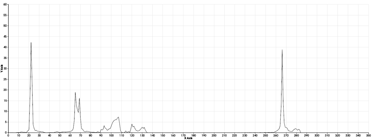 PCLPlotterクラスを用いてプロットしたVFHヒストグラム
生データ(浮動小数点のベクトルなど)がある場合は、addHistogramDat()関数を使用してヒストグラムとしてプロットすることができる。
- 入力: 記述子、記述子のサイズ, Descriptor, descriptor size,(ウィンドゥのサイズ), (背景色), (Y軸の範囲)
- Tutorial: PCLPlotter
- API: pcl::visualization::PCLPlotter
- Download
PCLビューワー¶
PCLに付随するこのプログラムにより、保存された記述子を視覚化できる。 内部的にはPCLPlotterを使用している。 このようにコマンドラインからビューワーを呼び出すことができるので便利である:
pcl_viewer <descriptor_file>
 PCLビューワーによって表示されるVFHヒストグラム
Go to root: PhD-3D-Object-Tracking
Links to articles:
PCL/OpenNI tutorial 0: The very basics
PCL/OpenNI tutorial 1: Installing and testing
PCL/OpenNI tutorial 2: Cloud processing (basic)
PCL/OpenNI tutorial 3: Cloud processing (advanced)
PCL/OpenNI tutorial 4: 3D object recognition (descriptors)
PCL/OpenNI tutorial 5: 3D object recognition (pipeline)
PCL/OpenNI troubleshooting